Supervised learning

In this chapter, we will move beyond statistical regression, and introduce some of the popular machine learning methods.

In the first code chunk, we load necessary R libraries that will be utilized throughout the chapter for various machine learning methods and data visualization.

Read previously saved data

The second chunk is dedicated to reading previously saved data and formulas from specified file paths, ensuring that the dataset and predefined formulas are available for subsequent analyses.

ObsData <- readRDS(file = "Data/machinelearning/rhcAnalytic.RDS")
levels(ObsData$Death)=c("No","Yes")
out.formula1 <- readRDS(file = "Data/machinelearning/form1.RDS")
out.formula2 <- readRDS(file = "Data/machinelearning/form2.RDS")

Ridge, LASSO, and Elastic net

The traditional regression models (e.g., linear regression, logistic regression) show poor model performance when

predictors are highly correlated or
there are many predictors

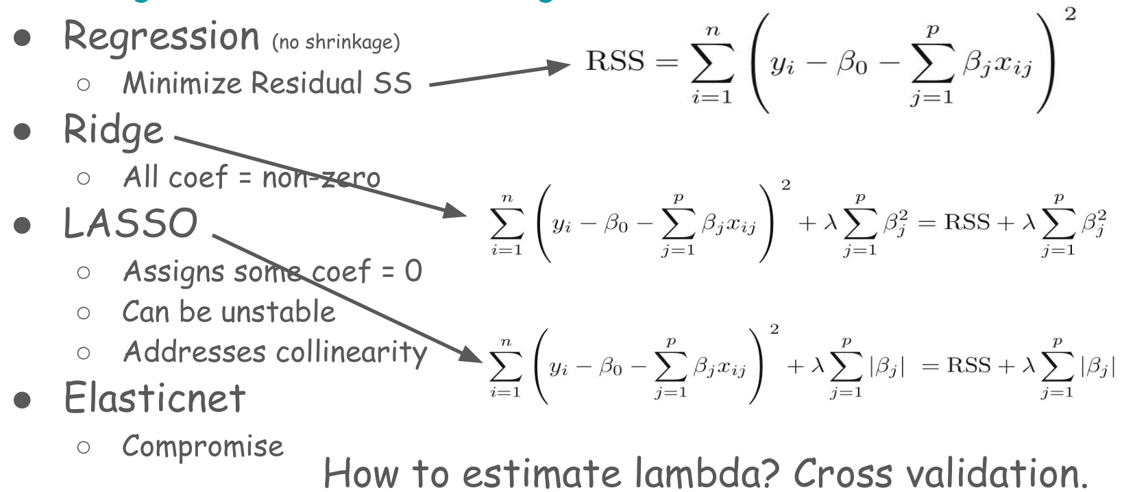
In both cases, the variance of the estimated regression coefficients could be highly variable. Hence, the model often results in poor predictions. The general solution to this problem is to reduce the variance at the cost of introducing some bias in the coefficients. This approach is called regularization or shrinking. Since we are interested in overall prediction rather than individual regression coefficients in a prediction context, this shrinkage approach is almost always beneficial for the model’s predictive performance. Ridge, LASSO, and Elastic Net are shrinkage machine learning techniques.

Ridge: Penalizes the sum of squared regression coefficients (the so-called \(L_2\) penalty). This approach does not remove irrelevant predictors, but minimizes the impact of the irrelevant predictors. There is a hyperparameter called \(\lambda\) (lambda) that determines the amount of shrinkage of the coefficients. The larger \(\lambda\) indicates more penalization of the coefficients.
LASSO: The Least Absolute Shrinkage and Selection Operator (LASSO) is quite similar conceptually to the ridge regression. However, lasso penalizes the sum of the absolute values of regression coefficients (so-called \(L_1\) penalty). As a result, a high \(\lambda\) value forces many coefficients to be exactly zero in lasso regression, suggesting a reduced model with fewer predictors, which is never the case in ridge regression.
Elastic Net: The elastic net combines the penalties of ridge regression and lasso to get the best of both methods. Two hyperparameters in the elastic net are \(\alpha\) (alpha) and \(\lambda\).

We can use the glmnet function in R to fit these there models.

Note

In glmnet function, alpha = 1 for the LASSO, alpha = 0 for the ridge, and setting alpha to some value between 0 and 1 is the elastic net model.

Continuous outcome

Cross-validation LASSO

In this code chunk, we implement a machine learning model training process with a focus on utilizing cross-validation and tuning parameters to optimize the model. Cross-validation is a technique used to assess how well the model will generalize to an independent dataset by partitioning the original dataset into a training set to train the model, and a test set to evaluate it. Here, we specify that we are using a particular type of cross-validation, denoted as “cv”, and that we will be creating 5 folds (or partitions) of the data, as indicated by number = 5.

The model being trained is specified to use a method known as “glmnet”, which is capable of performing lasso, ridge, and elastic net regularization regressions. Tuning parameters are crucial in controlling the behavior of our learning algorithm. In this instance, we specify lambda and alpha as our tuning parameters, which control the amount of regularization applied to the model and the mixing percentage between lasso and ridge regression, respectively. The tuneGrid argument is used to specify the exact values of alpha and lambda that the model should consider during training. Here we tune over a grid of positive lambda values so that cross-validation can actually select the amount of shrinkage (a single lambda = 0 would apply no penalty and simply recover the ordinary least squares fit). The verbose = FALSE argument ensures that additional model training details are not printed during the training process. Finally, the trained model is stored in an object for further examination and use.

ctrl <- trainControl(method = "cv", number = 5)
fit.cv.con <- train(out.formula1,
                    trControl = ctrl,
                    data = ObsData, method = "glmnet",
                    tuneGrid = expand.grid(alpha = 1,
                                           lambda = 10^seq(-4, 1, length = 50)),
                    verbose = FALSE)
#> Warning in nominalTrainWorkflow(x = x, y = y, wts = weights, info = trainInfo,
#> : There were missing values in resampled performance measures.
fit.cv.con
#> glmnet 
#> 
#> 5735 samples
#>   50 predictor
#> 
#> No pre-processing
#> Resampling: Cross-Validated (5 fold) 
#> Summary of sample sizes: 4589, 4587, 4588, 4588, 4588 
#> Resampling results across tuning parameters:
#> 
#>   lambda        RMSE      Rsquared    MAE     
#>   1.000000e-04  24.98173  0.06021230  15.15948
#>   1.264855e-04  24.98173  0.06021230  15.15948
#>   1.599859e-04  24.98173  0.06021230  15.15948
#>   2.023590e-04  24.98173  0.06021230  15.15948
#>   2.559548e-04  24.98173  0.06021230  15.15948
#>   3.237458e-04  24.98173  0.06021230  15.15948
#>   4.094915e-04  24.98173  0.06021230  15.15948
#>   5.179475e-04  24.98173  0.06021230  15.15948
#>   6.551286e-04  24.98173  0.06021230  15.15948
#>   8.286428e-04  24.98173  0.06021230  15.15948
#>   1.048113e-03  24.98173  0.06021230  15.15948
#>   1.325711e-03  24.98173  0.06021230  15.15948
#>   1.676833e-03  24.98173  0.06021230  15.15948
#>   2.120951e-03  24.98170  0.06021389  15.15935
#>   2.682696e-03  24.98153  0.06021977  15.15894
#>   3.393222e-03  24.98114  0.06023267  15.15805
#>   4.291934e-03  24.98064  0.06024766  15.15687
#>   5.428675e-03  24.98003  0.06026594  15.15539
#>   6.866488e-03  24.97927  0.06028799  15.15363
#>   8.685114e-03  24.97833  0.06031563  15.15148
#>   1.098541e-02  24.97718  0.06034932  15.14873
#>   1.389495e-02  24.97586  0.06038364  15.14531
#>   1.757511e-02  24.97433  0.06042067  15.14117
#>   2.222996e-02  24.97235  0.06047265  15.13611
#>   2.811769e-02  24.96953  0.06056579  15.12989
#>   3.556480e-02  24.96611  0.06068631  15.12298
#>   4.498433e-02  24.96210  0.06082935  15.11547
#>   5.689866e-02  24.95773  0.06097846  15.10689
#>   7.196857e-02  24.95335  0.06111854  15.09830
#>   9.102982e-02  24.94942  0.06122207  15.08935
#>   1.151395e-01  24.94571  0.06131902  15.07965
#>   1.456348e-01  24.94254  0.06141272  15.07106
#>   1.842070e-01  24.94170  0.06141400  15.06578
#>   2.329952e-01  24.94405  0.06129930  15.05873
#>   2.947052e-01  24.95311  0.06079563  15.05728
#>   3.727594e-01  24.96846  0.05999554  15.06658
#>   4.714866e-01  24.99549  0.05853464  15.09248
#>   5.963623e-01  25.03812  0.05609877  15.13807
#>   7.543120e-01  25.09467  0.05295167  15.19973
#>   9.540955e-01  25.14669  0.05096275  15.26115
#>   1.206793e+00  25.21234  0.04888299  15.34021
#>   1.526418e+00  25.30650  0.04527545  15.44342
#>   1.930698e+00  25.43380  0.03869498  15.58248
#>   2.442053e+00  25.58755  0.02209982  15.74909
#>   3.088844e+00  25.68147  0.01919278  15.85082
#>   3.906940e+00  25.72171         NaN  15.89151
#>   4.941713e+00  25.72171         NaN  15.89151
#>   6.250552e+00  25.72171         NaN  15.89151
#>   7.906043e+00  25.72171         NaN  15.89151
#>   1.000000e+01  25.72171         NaN  15.89151
#> 
#> Tuning parameter 'alpha' was held constant at a value of 1
#> RMSE was used to select the optimal model using the smallest value.
#> The final values used for the model were alpha = 1 and lambda = 0.184207.

Cross-validation Ridge

Subsequent code chunks explore Ridge regression and Elastic Net, employing similar methodologies but adjusting tuning parameters accordingly.

ctrl <- trainControl(method = "cv", number = 5)
fit.cv.con <-train(out.formula1,
                   trControl = ctrl,
                   data = ObsData, method = "glmnet",
                   tuneGrid = expand.grid(alpha = 0,
                                          lambda = 10^seq(-4, 1, length = 50)),
                   verbose = FALSE)
fit.cv.con
#> glmnet 
#> 
#> 5735 samples
#>   50 predictor
#> 
#> No pre-processing
#> Resampling: Cross-Validated (5 fold) 
#> Summary of sample sizes: 4587, 4589, 4588, 4589, 4587 
#> Resampling results across tuning parameters:
#> 
#>   lambda        RMSE      Rsquared    MAE     
#>   1.000000e-04  25.05686  0.06001154  15.14951
#>   1.264855e-04  25.05686  0.06001154  15.14951
#>   1.599859e-04  25.05686  0.06001154  15.14951
#>   2.023590e-04  25.05686  0.06001154  15.14951
#>   2.559548e-04  25.05686  0.06001154  15.14951
#>   3.237458e-04  25.05686  0.06001154  15.14951
#>   4.094915e-04  25.05686  0.06001154  15.14951
#>   5.179475e-04  25.05686  0.06001154  15.14951
#>   6.551286e-04  25.05686  0.06001154  15.14951
#>   8.286428e-04  25.05686  0.06001154  15.14951
#>   1.048113e-03  25.05686  0.06001154  15.14951
#>   1.325711e-03  25.05686  0.06001154  15.14951
#>   1.676833e-03  25.05686  0.06001154  15.14951
#>   2.120951e-03  25.05686  0.06001154  15.14951
#>   2.682696e-03  25.05686  0.06001154  15.14951
#>   3.393222e-03  25.05686  0.06001154  15.14951
#>   4.291934e-03  25.05686  0.06001154  15.14951
#>   5.428675e-03  25.05686  0.06001154  15.14951
#>   6.866488e-03  25.05686  0.06001154  15.14951
#>   8.685114e-03  25.05686  0.06001154  15.14951
#>   1.098541e-02  25.05686  0.06001154  15.14951
#>   1.389495e-02  25.05686  0.06001154  15.14951
#>   1.757511e-02  25.05686  0.06001154  15.14951
#>   2.222996e-02  25.05686  0.06001154  15.14951
#>   2.811769e-02  25.05686  0.06001154  15.14951
#>   3.556480e-02  25.05686  0.06001154  15.14951
#>   4.498433e-02  25.05686  0.06001154  15.14951
#>   5.689866e-02  25.05686  0.06001154  15.14951
#>   7.196857e-02  25.05686  0.06001154  15.14951
#>   9.102982e-02  25.05686  0.06001154  15.14951
#>   1.151395e-01  25.05686  0.06001154  15.14951
#>   1.456348e-01  25.05686  0.06001154  15.14951
#>   1.842070e-01  25.05686  0.06001154  15.14951
#>   2.329952e-01  25.05686  0.06001154  15.14951
#>   2.947052e-01  25.05686  0.06001154  15.14951
#>   3.727594e-01  25.05643  0.06001864  15.14821
#>   4.714866e-01  25.05501  0.06004207  15.14437
#>   5.963623e-01  25.05332  0.06006965  15.13991
#>   7.543120e-01  25.05129  0.06010447  15.13464
#>   9.540955e-01  25.04891  0.06014610  15.12857
#>   1.206793e+00  25.04615  0.06019508  15.12168
#>   1.526418e+00  25.04303  0.06025261  15.11399
#>   1.930698e+00  25.03965  0.06031553  15.10530
#>   2.442053e+00  25.03611  0.06038447  15.09595
#>   3.088844e+00  25.03274  0.06044847  15.08609
#>   3.906940e+00  25.02985  0.06050586  15.07615
#>   4.941713e+00  25.02796  0.06054741  15.06796
#>   6.250552e+00  25.02769  0.06056332  15.06270
#>   7.906043e+00  25.02984  0.06054186  15.06135
#>   1.000000e+01  25.03528  0.06047080  15.06476
#> 
#> Tuning parameter 'alpha' was held constant at a value of 0
#> RMSE was used to select the optimal model using the smallest value.
#> The final values used for the model were alpha = 0 and lambda = 6.250552.

Binary outcome

Cross-validation LASSO

We then shift to binary outcomes, exploring LASSO and Ridge regression with similar implementations but adjusting for the binary nature of the outcome variable.

ctrl<-trainControl(method = "cv", number = 5,
                   classProbs = TRUE,
                   summaryFunction = twoClassSummary)
fit.cv.bin<-train(out.formula2,
                  trControl = ctrl,
                  data = ObsData,
                  method = "glmnet",
                  tuneGrid = expand.grid(alpha = 1,
                                         lambda = 10^seq(-4, 1, length = 50)),
                  verbose = FALSE,
                  metric="ROC")
fit.cv.bin
#> glmnet 
#> 
#> 5735 samples
#>   50 predictor
#>    2 classes: 'No', 'Yes' 
#> 
#> No pre-processing
#> Resampling: Cross-Validated (5 fold) 
#> Summary of sample sizes: 4587, 4589, 4589, 4588, 4587 
#> Resampling results across tuning parameters:
#> 
#>   lambda        ROC        Sens          Spec     
#>   1.000000e-04  0.7554201  0.4639840500  0.8565371
#>   1.264855e-04  0.7554201  0.4639840500  0.8565371
#>   1.599859e-04  0.7554308  0.4639840500  0.8562683
#>   2.023590e-04  0.7554035  0.4634865375  0.8565371
#>   2.559548e-04  0.7553781  0.4624927472  0.8568059
#>   3.237458e-04  0.7553415  0.4624915127  0.8570748
#>   4.094915e-04  0.7552896  0.4614964878  0.8568056
#>   5.179475e-04  0.7552724  0.4605026974  0.8562680
#>   6.551286e-04  0.7551131  0.4580200733  0.8570737
#>   8.286428e-04  0.7549745  0.4575225609  0.8581489
#>   1.048113e-03  0.7550079  0.4560349617  0.8586862
#>   1.325711e-03  0.7549476  0.4550399368  0.8605672
#>   1.676833e-03  0.7548311  0.4515610533  0.8613730
#>   2.120951e-03  0.7545292  0.4485821513  0.8635228
#>   2.682696e-03  0.7544181  0.4441094774  0.8670149
#>   3.393222e-03  0.7543359  0.4391466983  0.8686267
#>   4.291934e-03  0.7543183  0.4336814686  0.8702371
#>   5.428675e-03  0.7537122  0.4247410590  0.8742682
#>   6.866488e-03  0.7526631  0.4138143032  0.8777614
#>   8.685114e-03  0.7507882  0.4013826648  0.8831327
#>   1.098541e-02  0.7488829  0.3730627261  0.8944165
#>   1.389495e-02  0.7461829  0.3447526635  0.9067760
#>   1.757511e-02  0.7415286  0.3000444428  0.9210154
#>   2.222996e-02  0.7336198  0.2473957755  0.9352533
#>   2.811769e-02  0.7229930  0.1793402713  0.9572848
#>   3.556480e-02  0.7151051  0.1097897609  0.9734037
#>   4.498433e-02  0.7091101  0.0427231090  0.9911341
#>   5.689866e-02  0.6985177  0.0009925558  0.9997315
#>   7.196857e-02  0.6874605  0.0000000000  1.0000000
#>   9.102982e-02  0.5808116  0.0000000000  1.0000000
#>   1.151395e-01  0.5000000  0.0000000000  1.0000000
#>   1.456348e-01  0.5000000  0.0000000000  1.0000000
#>   1.842070e-01  0.5000000  0.0000000000  1.0000000
#>   2.329952e-01  0.5000000  0.0000000000  1.0000000
#>   2.947052e-01  0.5000000  0.0000000000  1.0000000
#>   3.727594e-01  0.5000000  0.0000000000  1.0000000
#>   4.714866e-01  0.5000000  0.0000000000  1.0000000
#>   5.963623e-01  0.5000000  0.0000000000  1.0000000
#>   7.543120e-01  0.5000000  0.0000000000  1.0000000
#>   9.540955e-01  0.5000000  0.0000000000  1.0000000
#>   1.206793e+00  0.5000000  0.0000000000  1.0000000
#>   1.526418e+00  0.5000000  0.0000000000  1.0000000
#>   1.930698e+00  0.5000000  0.0000000000  1.0000000
#>   2.442053e+00  0.5000000  0.0000000000  1.0000000
#>   3.088844e+00  0.5000000  0.0000000000  1.0000000
#>   3.906940e+00  0.5000000  0.0000000000  1.0000000
#>   4.941713e+00  0.5000000  0.0000000000  1.0000000
#>   6.250552e+00  0.5000000  0.0000000000  1.0000000
#>   7.906043e+00  0.5000000  0.0000000000  1.0000000
#>   1.000000e+01  0.5000000  0.0000000000  1.0000000
#> 
#> Tuning parameter 'alpha' was held constant at a value of 1
#> ROC was used to select the optimal model using the largest value.
#> The final values used for the model were alpha = 1 and lambda = 0.0001599859.

Not okay to select variables from a shrinkage model, and then use them in a regular regression

Cross-validation Ridge

ctrl<-trainControl(method = "cv", number = 5,
                   classProbs = TRUE,
                   summaryFunction = twoClassSummary)
fit.cv.bin<-train(out.formula2, trControl = ctrl,
               data = ObsData, method = "glmnet",
               tuneGrid = expand.grid(alpha = 0,
                                      lambda = 10^seq(-4, 1, length = 50)),
               verbose = FALSE,
               metric="ROC")
fit.cv.bin
#> glmnet 
#> 
#> 5735 samples
#>   50 predictor
#>    2 classes: 'No', 'Yes' 
#> 
#> No pre-processing
#> Resampling: Cross-Validated (5 fold) 
#> Summary of sample sizes: 4589, 4588, 4587, 4587, 4589 
#> Resampling results across tuning parameters:
#> 
#>   lambda        ROC        Sens         Spec     
#>   1.000000e-04  0.7538395  0.450537634  0.8632431
#>   1.264855e-04  0.7538395  0.450537634  0.8632431
#>   1.599859e-04  0.7538395  0.450537634  0.8632431
#>   2.023590e-04  0.7538395  0.450537634  0.8632431
#>   2.559548e-04  0.7538395  0.450537634  0.8632431
#>   3.237458e-04  0.7538395  0.450537634  0.8632431
#>   4.094915e-04  0.7538395  0.450537634  0.8632431
#>   5.179475e-04  0.7538395  0.450537634  0.8632431
#>   6.551286e-04  0.7538395  0.450537634  0.8632431
#>   8.286428e-04  0.7538395  0.450537634  0.8632431
#>   1.048113e-03  0.7538395  0.450537634  0.8632431
#>   1.325711e-03  0.7538395  0.450537634  0.8632431
#>   1.676833e-03  0.7538395  0.450537634  0.8632431
#>   2.120951e-03  0.7538395  0.450537634  0.8632431
#>   2.682696e-03  0.7538395  0.450537634  0.8632431
#>   3.393222e-03  0.7538395  0.450537634  0.8632431
#>   4.291934e-03  0.7538395  0.450537634  0.8632431
#>   5.428675e-03  0.7538395  0.450537634  0.8632431
#>   6.866488e-03  0.7538395  0.450537634  0.8632431
#>   8.685114e-03  0.7538395  0.450537634  0.8632431
#>   1.098541e-02  0.7537514  0.448053776  0.8640496
#>   1.389495e-02  0.7535705  0.443086059  0.8664682
#>   1.757511e-02  0.7534170  0.440107157  0.8672747
#>   2.222996e-02  0.7532248  0.433651840  0.8688872
#>   2.811769e-02  0.7529892  0.426201499  0.8710356
#>   3.556480e-02  0.7525827  0.416766046  0.8742596
#>   4.498433e-02  0.7521254  0.405838055  0.8793639
#>   5.689866e-02  0.7515507  0.393417528  0.8868871
#>   7.196857e-02  0.7509401  0.382488303  0.8930656
#>   9.102982e-02  0.7501439  0.368083898  0.9011261
#>   1.151395e-01  0.7493755  0.349700628  0.9113354
#>   1.456348e-01  0.7483673  0.323385554  0.9207393
#>   1.842070e-01  0.7473569  0.294081701  0.9322916
#>   2.329952e-01  0.7461759  0.262792736  0.9406199
#>   2.947052e-01  0.7449967  0.222058442  0.9540539
#>   3.727594e-01  0.7437458  0.176361369  0.9674872
#>   4.714866e-01  0.7423924  0.134629582  0.9790413
#>   5.963623e-01  0.7409952  0.098372900  0.9887144
#>   7.543120e-01  0.7397328  0.055152278  0.9959699
#>   9.540955e-01  0.7384724  0.018883251  0.9994624
#>   1.206793e+00  0.7373235  0.003476414  1.0000000
#>   1.526418e+00  0.7363039  0.000000000  1.0000000
#>   1.930698e+00  0.7354312  0.000000000  1.0000000
#>   2.442053e+00  0.7345345  0.000000000  1.0000000
#>   3.088844e+00  0.7337665  0.000000000  1.0000000
#>   3.906940e+00  0.7330925  0.000000000  1.0000000
#>   4.941713e+00  0.7325848  0.000000000  1.0000000
#>   6.250552e+00  0.7321423  0.000000000  1.0000000
#>   7.906043e+00  0.7317560  0.000000000  1.0000000
#>   1.000000e+01  0.7314491  0.000000000  1.0000000
#> 
#> Tuning parameter 'alpha' was held constant at a value of 0
#> ROC was used to select the optimal model using the largest value.
#> The final values used for the model were alpha = 0 and lambda = 0.008685114.

Cross-validation Elastic net

Alpha = mixing parameter
Lambda = regularization or tuning parameter
We can use expand.grid for model tuning

ctrl<-trainControl(method = "cv", number = 5,
                   classProbs = TRUE,
                   summaryFunction = twoClassSummary)
fit.cv.bin<-train(out.formula2, trControl = ctrl,
               data = ObsData, method = "glmnet",
               tuneGrid = expand.grid(alpha = seq(0.1,.2,by = 0.05),  
                                      lambda = seq(0.05,0.3,by = 0.05)),
               verbose = FALSE,
               metric="ROC")
fit.cv.bin
#> glmnet 
#> 
#> 5735 samples
#>   50 predictor
#>    2 classes: 'No', 'Yes' 
#> 
#> No pre-processing
#> Resampling: Cross-Validated (5 fold) 
#> Summary of sample sizes: 4589, 4588, 4587, 4588, 4588 
#> Resampling results across tuning parameters:
#> 
#>   alpha  lambda  ROC        Sens          Spec     
#>   0.10   0.05    0.7501508  0.3661247114  0.8981789
#>   0.10   0.10    0.7468010  0.2747132822  0.9374017
#>   0.10   0.15    0.7417450  0.1758589188  0.9674937
#>   0.10   0.20    0.7363601  0.0874263916  0.9862983
#>   0.10   0.25    0.7300909  0.0258249694  0.9965079
#>   0.10   0.30    0.7233685  0.0009925558  0.9997312
#>   0.15   0.05    0.7492697  0.3437650457  0.9070455
#>   0.15   0.10    0.7422014  0.2205696085  0.9511056
#>   0.15   0.15    0.7335331  0.1023332469  0.9830739
#>   0.15   0.20    0.7226744  0.0188733751  0.9967764
#>   0.15   0.25    0.7152975  0.0000000000  1.0000000
#>   0.15   0.30    0.7098185  0.0000000000  1.0000000
#>   0.20   0.05    0.7476579  0.3229053245  0.9148355
#>   0.20   0.10    0.7367101  0.1679061269  0.9669564
#>   0.20   0.15    0.7223293  0.0382454971  0.9914029
#>   0.20   0.20    0.7125355  0.0004962779  0.9994627
#>   0.20   0.25    0.7062552  0.0000000000  1.0000000
#>   0.20   0.30    0.6962746  0.0000000000  1.0000000
#> 
#> ROC was used to select the optimal model using the largest value.
#> The final values used for the model were alpha = 0.1 and lambda = 0.05.
plot(fit.cv.bin)

Decision tree

Decision trees are then introduced and implemented, with visualizations and evaluation metrics provided to assess their performance.

Decision tree
- Referred to as Classification and regression trees or CART
- Covers
  - Classification (categorical outcome)
  - Regression (continuous outcome)
- Flexible to incorporate non-linear effects automatically
  - No need to specify higher order terms / interactions
- Unstable, prone to overfitting, suffers from high variance

Simple CART

Note

The AUC values reported for the CART models below are computed on the same data used to fit the trees, so they are apparent (optimistic) estimates of discrimination. The cross-validation chunks in this chapter give less biased estimates of out-of-sample performance.

require(rpart)
summary(ObsData$DASIndex) # Duke Activity Status Index
#>    Min. 1st Qu.  Median    Mean 3rd Qu.    Max. 
#>   11.00   16.06   19.75   20.50   23.43   33.00
cart.fit <- rpart(Death~DASIndex, data = ObsData)
par(mfrow = c(1,1), xpd = NA)
plot(cart.fit)
text(cart.fit, use.n = TRUE)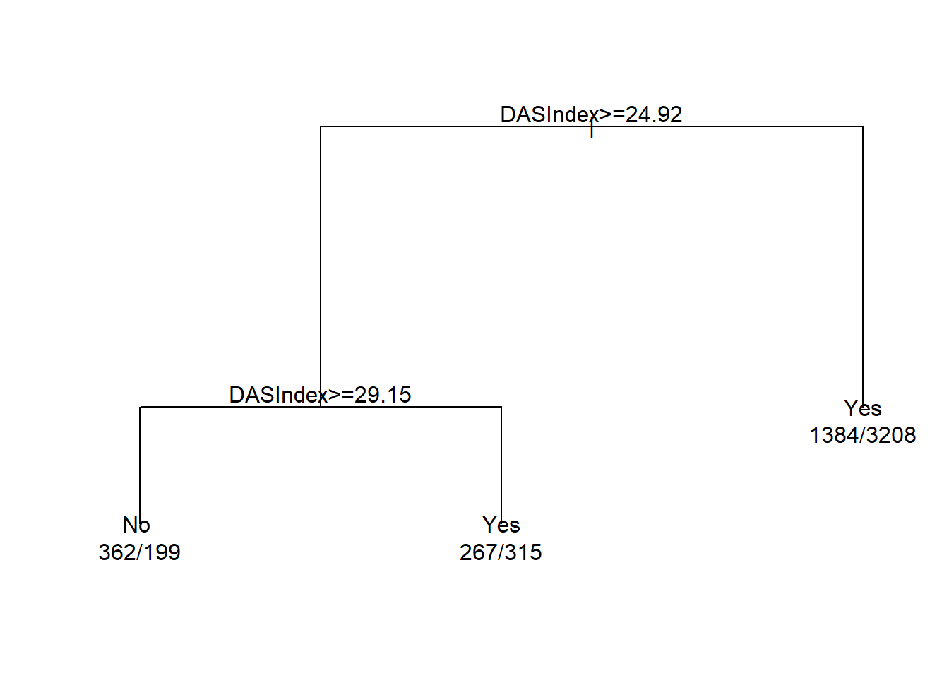

print(cart.fit)
#> n= 5735 
#> 
#> node), split, n, loss, yval, (yprob)
#>       * denotes terminal node
#> 
#> 1) root 5735 2013 Yes (0.3510026 0.6489974)  
#>   2) DASIndex>=24.92383 1143  514 No (0.5503062 0.4496938)  
#>     4) DASIndex>=29.14648 561  199 No (0.6452763 0.3547237) *
#>     5) DASIndex< 29.14648 582  267 Yes (0.4587629 0.5412371) *
#>   3) DASIndex< 24.92383 4592 1384 Yes (0.3013937 0.6986063) *
require(rattle)
require(rpart.plot)
require(RColorBrewer)
fancyRpartPlot(cart.fit, caption = NULL)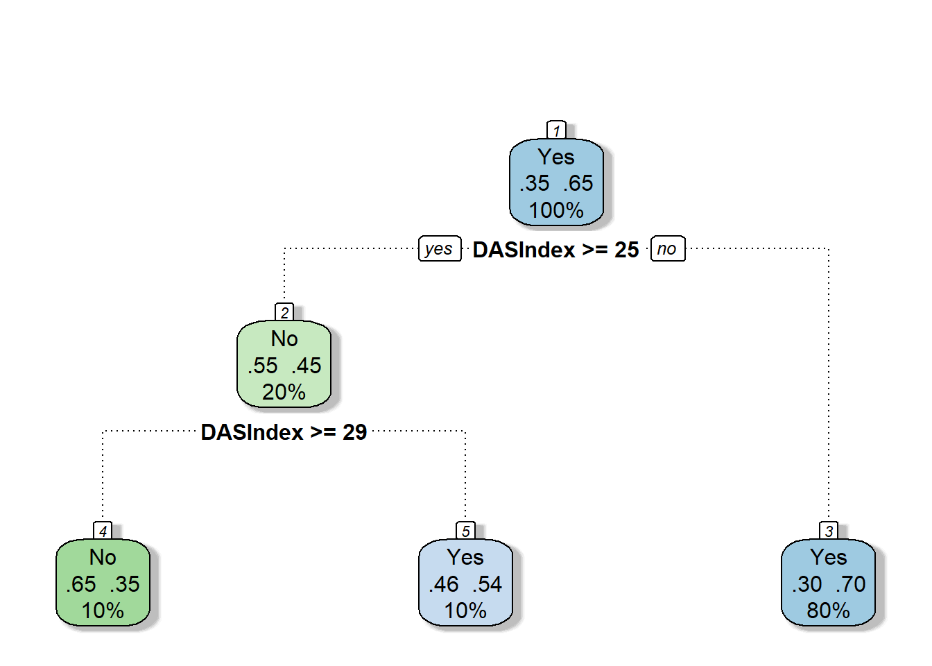

AUC

require(pROC)
#> Loading required package: pROC
#> Type 'citation("pROC")' for a citation.
#> 
#> Attaching package: 'pROC'
#> The following objects are masked from 'package:stats':
#> 
#>     cov, smooth, var
obs.y2<-ObsData$Death
pred.y2 <- as.numeric(predict(cart.fit, type = "prob")[, 2])
rocobj <- roc(obs.y2, pred.y2)
#> Setting levels: control = No, case = Yes
#> Setting direction: controls < cases
rocobj
#> 
#> Call:
#> roc.default(response = obs.y2, predictor = pred.y2)
#> 
#> Data: pred.y2 in 2013 controls (obs.y2 No) < 3722 cases (obs.y2 Yes).
#> Area under the curve: 0.5912
plot(rocobj)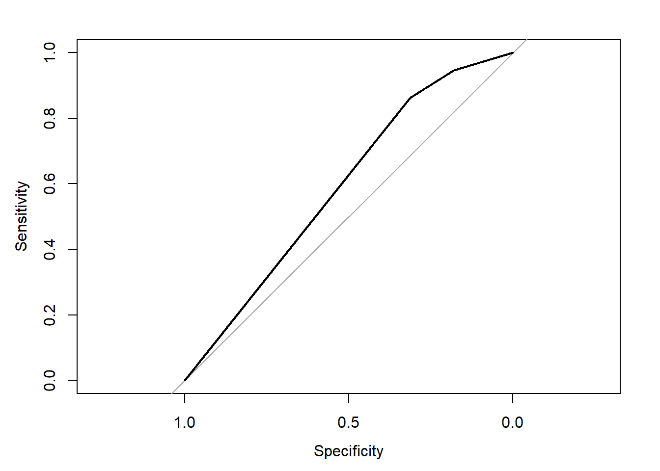

auc(rocobj)
#> Area under the curve: 0.5912

Complex CART

More variables

out.formula2
#> Death ~ Disease.category + Cancer + Cardiovascular + Congestive.HF + 
#>     Dementia + Psychiatric + Pulmonary + Renal + Hepatic + GI.Bleed + 
#>     Tumor + Immunosupperssion + Transfer.hx + MI + age + sex + 
#>     edu + DASIndex + APACHE.score + Glasgow.Coma.Score + blood.pressure + 
#>     WBC + Heart.rate + Respiratory.rate + Temperature + PaO2vs.FIO2 + 
#>     Albumin + Hematocrit + Bilirubin + Creatinine + Sodium + 
#>     Potassium + PaCo2 + PH + Weight + DNR.status + Medical.insurance + 
#>     Respiratory.Diag + Cardiovascular.Diag + Neurological.Diag + 
#>     Gastrointestinal.Diag + Renal.Diag + Metabolic.Diag + Hematologic.Diag + 
#>     Sepsis.Diag + Trauma.Diag + Orthopedic.Diag + race + income + 
#>     RHC.use
require(rpart)
cart.fit <- rpart(out.formula2, data = ObsData)

CART Variable importance

cart.fit$variable.importance
#>            DASIndex              Cancer               Tumor                 age 
#>         123.2102455          33.4559400          32.5418433          24.0804860 
#>   Medical.insurance                 WBC                 edu Cardiovascular.Diag 
#>          14.5199953           5.6673997           3.7441554           3.6449371 
#>          Heart.rate      Cardiovascular         Trauma.Diag               PaCo2 
#>           3.4059248           3.1669125           0.5953098           0.2420672 
#>           Potassium              Sodium             Albumin 
#>           0.2420672           0.2420672           0.1984366

AUC

require(pROC)
obs.y2<-ObsData$Death
pred.y2 <- as.numeric(predict(cart.fit, type = "prob")[, 2])
rocobj <- roc(obs.y2, pred.y2)
#> Setting levels: control = No, case = Yes
#> Setting direction: controls < cases
rocobj
#> 
#> Call:
#> roc.default(response = obs.y2, predictor = pred.y2)
#> 
#> Data: pred.y2 in 2013 controls (obs.y2 No) < 3722 cases (obs.y2 Yes).
#> Area under the curve: 0.5981
plot(rocobj)

auc(rocobj)
#> Area under the curve: 0.5981

Cross-validation CART

set.seed(504)
require(caret)
ctrl<-trainControl(method = "cv", number = 5, 
                   classProbs = TRUE,
                   summaryFunction = twoClassSummary)
# fit the model with formula = out.formula2
fit.cv.bin<-train(out.formula2, trControl = ctrl,
               data = ObsData, method = "rpart",
              metric="ROC")
fit.cv.bin
#> CART 
#> 
#> 5735 samples
#>   50 predictor
#>    2 classes: 'No', 'Yes' 
#> 
#> No pre-processing
#> Resampling: Cross-Validated (5 fold) 
#> Summary of sample sizes: 4587, 4589, 4587, 4589, 4588 
#> Resampling results across tuning parameters:
#> 
#>   cp           ROC        Sens       Spec     
#>   0.007203179  0.6304911  0.2816488  0.9086574
#>   0.039741679  0.5725283  0.2488649  0.8981807
#>   0.057128664  0.5380544  0.1287804  0.9473284
#> 
#> ROC was used to select the optimal model using the largest value.
#> The final value used for the model was cp = 0.007203179.
# extract results from each test data 
summary.res <- fit.cv.bin$resample
summary.res

Ensemble methods (Type I)

We explore ensemble methods, specifically bagging and boosting, through implementation and evaluation in the context of binary outcomes.

Training same model to different samples (of the same data)

Cross-validation bagging

Bagging or bootstrap aggregation
- independent bootstrap samples (sampling with replacement, B times),
- applies CART on each i (no prunning)
- Average the resulting predictions
- Reduces variance as a result of using bootstrap

set.seed(504)
require(caret)
ctrl<-trainControl(method = "cv", number = 5,
                   classProbs = TRUE,
                   summaryFunction = twoClassSummary)
# fit the model with formula = out.formula2
fit.cv.bin<-train(out.formula2, trControl = ctrl,
               data = ObsData, method = "bag",
               bagControl = bagControl(fit = ldaBag$fit, 
                                       predict = ldaBag$pred, 
                                       aggregate = ldaBag$aggregate),
               metric="ROC")
#> Warning: executing %dopar% sequentially: no parallel backend registered
fit.cv.bin
#> Bagged Model 
#> 
#> 5735 samples
#>   50 predictor
#>    2 classes: 'No', 'Yes' 
#> 
#> No pre-processing
#> Resampling: Cross-Validated (5 fold) 
#> Summary of sample sizes: 4587, 4589, 4587, 4589, 4588 
#> Resampling results:
#> 
#>   ROC        Sens       Spec     
#>   0.7506666  0.4485809  0.8602811
#> 
#> Tuning parameter 'vars' was held constant at a value of 63

Bagging improves prediction accuracy
- over prediction using a single tree
Looses interpretability
- as this is an average of many diagrams now
But we can get a summary of the importance of each variable

Bagging Variable importance

caret::varImp(fit.cv.bin, scale = FALSE)
#> ROC curve variable importance
#> 
#>   only 20 most important variables shown (out of 50)
#> 
#>                    Importance
#> age                    0.6159
#> APACHE.score           0.6140
#> DASIndex               0.5962
#> Cancer                 0.5878
#> Creatinine             0.5835
#> Tumor                  0.5807
#> blood.pressure         0.5697
#> Glasgow.Coma.Score     0.5656
#> Disease.category       0.5641
#> Temperature            0.5584
#> DNR.status             0.5572
#> Hematocrit             0.5525
#> Weight                 0.5424
#> Bilirubin              0.5397
#> income                 0.5319
#> Immunosupperssion      0.5278
#> RHC.use                0.5263
#> Dementia               0.5252
#> Congestive.HF          0.5250
#> Hematologic.Diag       0.5250

Cross-validation boosting

Boosting
- sequentially updated/weighted bootstrap based on previous learning

set.seed(504)
require(caret)
ctrl<-trainControl(method = "cv", number = 5,
                   classProbs = TRUE,
                   summaryFunction = twoClassSummary)
# fit the model with formula = out.formula2
fit.cv.bin<-train(out.formula2, trControl = ctrl,
               data = ObsData, method = "gbm",
               verbose = FALSE,
               metric="ROC")
fit.cv.bin
#> Stochastic Gradient Boosting 
#> 
#> 5735 samples
#>   50 predictor
#>    2 classes: 'No', 'Yes' 
#> 
#> No pre-processing
#> Resampling: Cross-Validated (5 fold) 
#> Summary of sample sizes: 4587, 4589, 4587, 4589, 4588 
#> Resampling results across tuning parameters:
#> 
#>   interaction.depth  n.trees  ROC        Sens       Spec     
#>   1                   50      0.7218938  0.2145970  0.9505647
#>   1                  100      0.7410292  0.2980581  0.9234228
#>   1                  150      0.7483014  0.3487142  0.9030028
#>   2                   50      0.7414513  0.2960631  0.9263816
#>   2                  100      0.7534264  0.3869684  0.8917212
#>   2                  150      0.7575826  0.4187512  0.8777477
#>   3                   50      0.7496078  0.3626125  0.9070358
#>   3                  100      0.7579645  0.4078244  0.8764076
#>   3                  150      0.7637074  0.4445909  0.8702298
#> 
#> Tuning parameter 'shrinkage' was held constant at a value of 0.1
#> 
#> Tuning parameter 'n.minobsinnode' was held constant at a value of 10
#> ROC was used to select the optimal model using the largest value.
#> The final values used for the model were n.trees = 150, interaction.depth =
#>  3, shrinkage = 0.1 and n.minobsinnode = 10.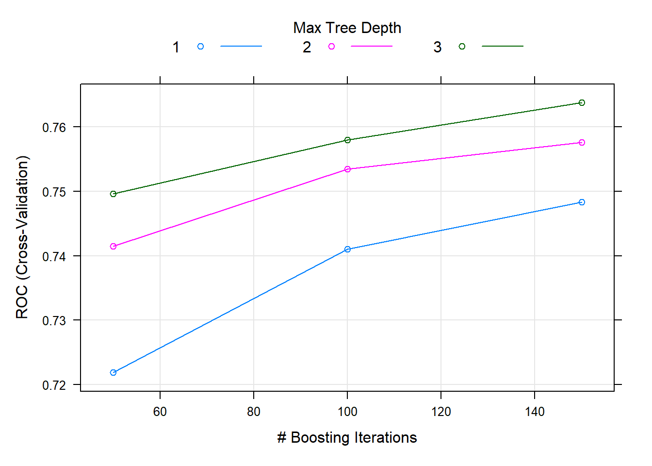

plot(fit.cv.bin)

Ensemble methods (Type II)

We introduce the concept of Super Learner, providing external resources for further exploration.

Training different models on the same data

Super Learner

Large number of candidate learners (CL) with different strengths
- Parametric (logistic)
- Non-parametric (CART)
Cross-validation: CL applied on training data, prediction made on test data
Final prediction uses a weighted version of all predictions
- Weights = coef of Observed outcome ~ prediction from each CL
- The weights are estimated under a convex-combination constraint: they are non-negative and sum to one (e.g., SuperLearner’s method.NNLS for continuous outcomes or method.NNloglik for binary outcomes), so the ensemble prediction is a weighted average of the candidate learners’ predictions.

Steps

Refer to this tutorial for steps and examples! Refer to the next chapter for more details.

Video content (optional)

Tip

For those who prefer a video walkthrough, feel free to watch the video below, which offers a description of an earlier version of the above content.

Tip

The following is a brief exercise of super learners in the propensity score context, but we will explore more about this topic in the next chapter.