Binary outcome
This tutorial is very similar to one of the previous tutorials, but uses a different data (we used RHC data here). We are revisiting concepts related to prediction before introducing ideas related to machine learning.
In this chapter, we will talk about Regression that deals with prediction of binary outcomes. We will use logistic regression to build the first prediction model.
Read previously saved data
Outcome levels (factor)
- Label
- Possible values of outcome
Measuring prediction error
-
Brier score
- Brier score 0 means perfect prediction, and
- close to zero means better prediction,
- 1 being the worst prediction.
- Less accurate forecasts get higher score in Brier score.
-
AUC
- The area under a ROC curve is called as a c statistics.
- c being 0.5 means random prediction and
- 1 indicates perfect prediction
Prediction for death
In this section, we show the regression fitting when outcome is binary (death).
Variables
baselinevars <- names(dplyr::select(ObsData,
                         !c(Length.of.Stay,Death)))
baselinevars
#>  [1] "Disease.category"      "Cancer"                "Cardiovascular"
#>  [4] "Congestive.HF"         "Dementia"              "Psychiatric"
#>  [7] "Pulmonary"             "Renal"                 "Hepatic"
#> [10] "GI.Bleed"              "Tumor"                 "Immunosupperssion"
#> [13] "Transfer.hx"           "MI"                    "age"
#> [16] "sex"                   "edu"                   "DASIndex"
#> [19] "APACHE.score"          "Glasgow.Coma.Score"    "blood.pressure"
#> [22] "WBC"                   "Heart.rate"            "Respiratory.rate"
#> [25] "Temperature"           "PaO2vs.FIO2"           "Albumin"
#> [28] "Hematocrit"            "Bilirubin"             "Creatinine"
#> [31] "Sodium"                "Potassium"             "PaCo2"
#> [34] "PH"                    "Weight"                "DNR.status"
#> [37] "Medical.insurance"     "Respiratory.Diag"      "Cardiovascular.Diag"
#> [40] "Neurological.Diag"     "Gastrointestinal.Diag" "Renal.Diag"
#> [43] "Metabolic.Diag"        "Hematologic.Diag"      "Sepsis.Diag"
#> [46] "Trauma.Diag"           "Orthopedic.Diag"       "race"
#> [49] "income"                "RHC.use"
Model
# adjust covariates
out.formula2 <- as.formula(paste("Death~ ", paste(baselinevars, collapse = "+")))
saveRDS(out.formula2, file = "Data/machinelearning/form2.RDS")
fit2 <- glm(out.formula2, data = ObsData,
            family = binomial(link = "logit"))
require(Publish)
adj.fit2 <- publish(fit2, digits=1)$regressionTable
out.formula2
#> Death ~ Disease.category + Cancer + Cardiovascular + Congestive.HF +
#> Dementia + Psychiatric + Pulmonary + Renal + Hepatic + GI.Bleed +
#> Tumor + Immunosupperssion + Transfer.hx + MI + age + sex +
#> edu + DASIndex + APACHE.score + Glasgow.Coma.Score + blood.pressure +
#> WBC + Heart.rate + Respiratory.rate + Temperature + PaO2vs.FIO2 +
#> Albumin + Hematocrit + Bilirubin + Creatinine + Sodium +
#> Potassium + PaCo2 + PH + Weight + DNR.status + Medical.insurance +
#> Respiratory.Diag + Cardiovascular.Diag + Neurological.Diag +
#> Gastrointestinal.Diag + Renal.Diag + Metabolic.Diag + Hematologic.Diag +
#> Sepsis.Diag + Trauma.Diag + Orthopedic.Diag + race + income +
#> RHC.use
adj.fit2Measuring prediction error
The AUC and Brier score below are computed on the same data used to fit the model (no newdata, no split or cross-validation). They are therefore apparent (optimistic) performance estimates. The cross-validation and data-splitting approaches shown later in this module, and the optimism correction in predictivefactors7, give less biased estimates of out-of-sample performance.
AUC
require(pROC)
#> Loading required package: pROC
#> Type 'citation("pROC")' for a citation.
#>
#> Attaching package: 'pROC'
#> The following objects are masked from 'package:stats':
#>
#>     cov, smooth, var
obs.y2<-ObsData$Death
pred.y2 <- predict(fit2, type = "response")
rocobj <- roc(obs.y2, pred.y2)
#> Setting levels: control = No, case = Yes
#> Setting direction: controls < cases
rocobj
#>
#> Call:
#> roc.default(response = obs.y2, predictor = pred.y2)
#>
#> Data: pred.y2 in 2013 controls (obs.y2 No) < 3722 cases (obs.y2 Yes).
#> Area under the curve: 0.7682
plot(rocobj)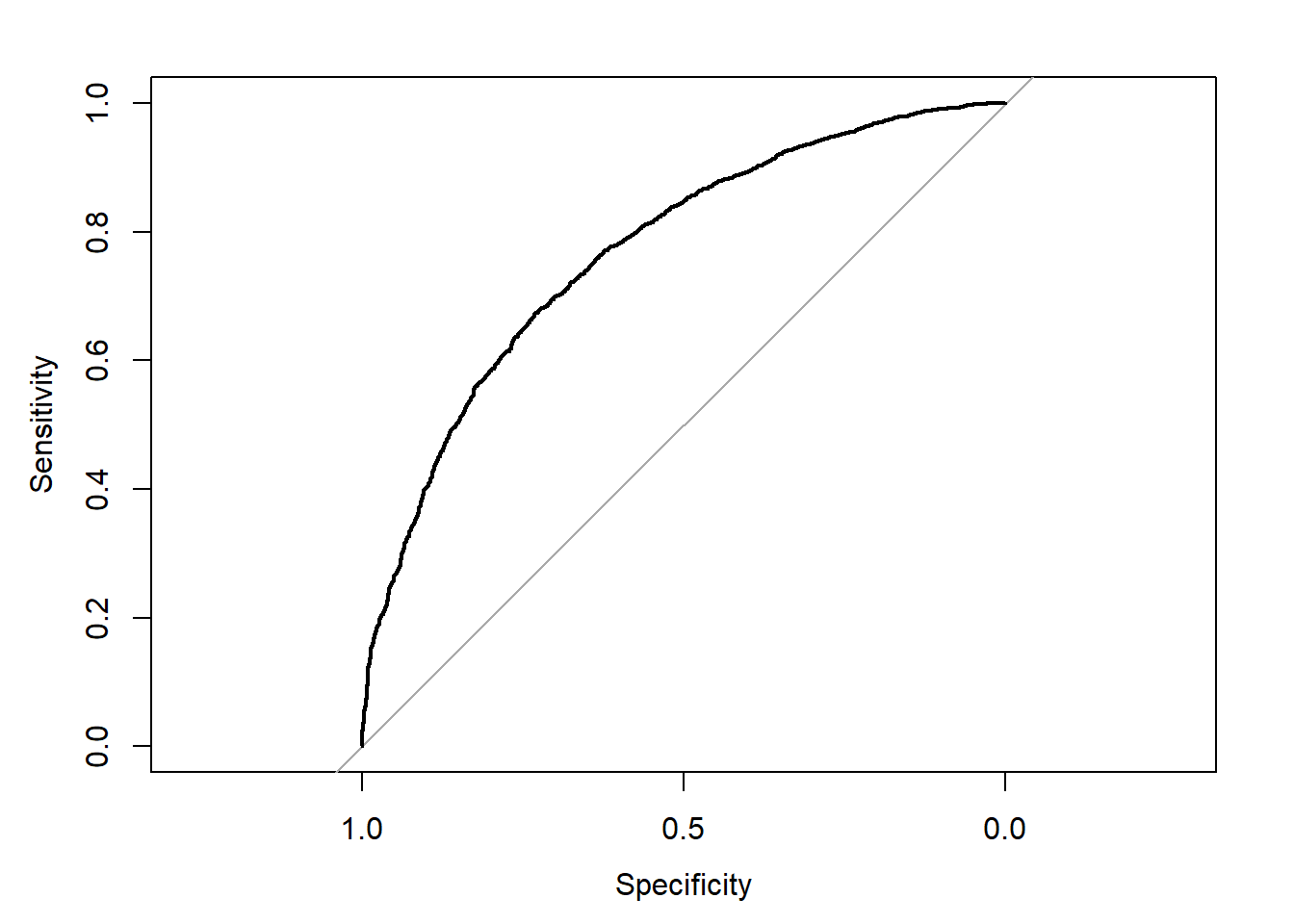
Brier Score
Cross-validation using caret
Basic setup
# Using Caret package
set.seed(504)

# make a 5-fold CV
require(caret)
#> Loading required package: caret
#> Loading required package: ggplot2
#> Loading required package: lattice
#>
#> Attaching package: 'caret'
#> The following objects are masked from 'package:DescTools':
#>
#>     MAE, RMSE
ctrl<-trainControl(method = "cv", number = 5,
                   classProbs = TRUE,
                   summaryFunction = twoClassSummary)

# fit the model with formula = out.formula2
# use training method glm (have to specify family)
fit.cv.bin<-train(out.formula2, trControl = ctrl,
               data = ObsData, method = "glm",
              family = binomial(),
              metric="ROC")
fit.cv.bin
#> Generalized Linear Model
#>
#> 5735 samples
#>   50 predictor
#>    2 classes: 'No', 'Yes'
#>
#> No pre-processing
#> Resampling: Cross-Validated (5 fold)
#> Summary of sample sizes: 4587, 4589, 4587, 4589, 4588
#> Resampling results:
#>
#>   ROC        Sens       Spec
#>   0.7545115  0.4659618  0.8535653
Extract results from each test data
More options
ctrl<-trainControl(method = "cv", number = 5,
                   classProbs = TRUE,
                   summaryFunction = twoClassSummary)
fit.cv.bin<-train(out.formula2, trControl = ctrl,
               data = ObsData, method = "glm",
              family = binomial(),
              metric="ROC",
              preProc = c("center", "scale"))
fit.cv.bin
#> Generalized Linear Model
#>
#> 5735 samples
#>   50 predictor
#>    2 classes: 'No', 'Yes'
#>
#> Pre-processing: centered (63), scaled (63)
#> Resampling: Cross-Validated (5 fold)
#> Summary of sample sizes: 4588, 4589, 4587, 4588, 4588
#> Resampling results:
#>
#>   ROC        Sens       Spec
#>   0.7548047  0.4629717  0.8530367
Variable selection
We can also use stepwise regression that uses AIC as a criterion.
fit.cv.bin.aic
#> Generalized Linear Model with Stepwise Feature Selection
#>
#> 5735 samples
#>   50 predictor
#>    2 classes: 'No', 'Yes'
#>
#> No pre-processing
#> Resampling: Cross-Validated (5 fold)
#> Summary of sample sizes: 4587, 4589, 4587, 4589, 4588
#> Resampling results:
#>
#>   ROC        Sens      Spec
#>   0.7540424  0.464468  0.8562535
summary(fit.cv.bin.aic)
#>
#> Call:
#> NULL
#>
#> Coefficients:
#>                                          Estimate Std. Error z value Pr(>|z|)
#> (Intercept)                             1.0783624  0.7822168   1.379 0.168019
#> Disease.categoryOther                   0.4495099  0.0919860   4.887 1.03e-06
#> `CancerLocalized (Yes)`                 1.8942512  0.5501880   3.443 0.000575
#> CancerMetastatic                        3.2703316  0.5858715   5.582 2.38e-08
#> Cardiovascular1                         0.2386749  0.0939617   2.540 0.011081
#> Congestive.HF1                          0.4539010  0.0971624   4.672 2.99e-06
#> Dementia1                               0.2380213  0.1162903   2.047 0.040679
#> Hepatic1                                0.3593093  0.1541762   2.331 0.019779
#> Tumor1                                 -1.2455123  0.5542624  -2.247 0.024630
#> Immunosupperssion1                      0.2174294  0.0730803   2.975 0.002928
#> Transfer.hx1                           -0.1849029  0.0945679  -1.955 0.050555
#> `age[50,60)`                            0.3621248  0.0984288   3.679 0.000234
#> `age[60,70)`                            0.6941924  0.0968434   7.168 7.60e-13
#> `age[70,80)`                            0.6804939  0.1126637   6.040 1.54e-09
#> `age[80, Inf)`                          0.9833851  0.1410563   6.972 3.13e-12
#> sexFemale                              -0.2805950  0.0653527  -4.294 1.76e-05
#> DASIndex                               -0.0429272  0.0062191  -6.902 5.11e-12
#> APACHE.score                            0.0174907  0.0020017   8.738  < 2e-16
#> Glasgow.Coma.Score                      0.0093657  0.0012563   7.455 9.00e-14
#> WBC                                     0.0044518  0.0030090   1.479 0.139009
#> Temperature                            -0.0524703  0.0192757  -2.722 0.006487
#> PaO2vs.FIO2                             0.0004741  0.0003054   1.552 0.120548
#> Hematocrit                             -0.0154796  0.0041593  -3.722 0.000198
#> Bilirubin                               0.0313087  0.0094004   3.331 0.000867
#> Weight                                 -0.0031548  0.0011213  -2.813 0.004902
#> DNR.statusYes                           0.9347360  0.1326924   7.044 1.86e-12
#> Medical.insuranceMedicare               0.4764895  0.1257582   3.789 0.000151
#> `Medical.insuranceMedicare & Medicaid`  0.3364916  0.1584757   2.123 0.033729
#> `Medical.insuranceNo insurance`         0.3711345  0.1568820   2.366 0.017996
#> Medical.insurancePrivate                0.2632637  0.1139805   2.310 0.020903
#> `Medical.insurancePrivate & Medicare`   0.2819715  0.1313101   2.147 0.031764
#> Respiratory.DiagYes                     0.1393974  0.0769026   1.813 0.069886
#> Cardiovascular.DiagYes                  0.1804967  0.0836679   2.157 0.030982
#> Neurological.DiagYes                    0.4320266  0.1189357   3.632 0.000281
#> Gastrointestinal.DiagYes                0.2819563  0.1092206   2.582 0.009836
#> Hematologic.DiagYes                     0.9734424  0.1651363   5.895 3.75e-09
#> Sepsis.DiagYes                          0.1539651  0.0943235   1.632 0.102614
#> `incomeUnder $11k`                      0.2151437  0.0689392   3.121 0.001804
#> RHC.use                                 0.3552053  0.0713632   4.977 6.44e-07
#>
#> (Intercept)
#> Disease.categoryOther                  ***
#> `CancerLocalized (Yes)`                ***
#> CancerMetastatic                       ***
#> Cardiovascular1                        *
#> Congestive.HF1                         ***
#> Dementia1                              *
#> Hepatic1                               *
#> Tumor1                                 *
#> Immunosupperssion1                     **
#> Transfer.hx1                           .
#> `age[50,60)`                           ***
#> `age[60,70)`                           ***
#> `age[70,80)`                           ***
#> `age[80, Inf)`                         ***
#> sexFemale                              ***
#> DASIndex                               ***
#> APACHE.score                           ***
#> Glasgow.Coma.Score                     ***
#> WBC
#> Temperature                            **
#> PaO2vs.FIO2
#> Hematocrit                             ***
#> Bilirubin                              ***
#> Weight                                 **
#> DNR.statusYes                          ***
#> Medical.insuranceMedicare              ***
#> `Medical.insuranceMedicare & Medicaid` *
#> `Medical.insuranceNo insurance`        *
#> Medical.insurancePrivate               *
#> `Medical.insurancePrivate & Medicare`  *
#> Respiratory.DiagYes                    .
#> Cardiovascular.DiagYes                 *
#> Neurological.DiagYes                   ***
#> Gastrointestinal.DiagYes               **
#> Hematologic.DiagYes                    ***
#> Sepsis.DiagYes
#> `incomeUnder $11k`                     **
#> RHC.use                                ***
#> ---
#> Signif. codes:  0 '***' 0.001 '**' 0.01 '*' 0.05 '.' 0.1 ' ' 1
#>
#> (Dispersion parameter for binomial family taken to be 1)
#>
#>     Null deviance: 7433.3  on 5734  degrees of freedom
#> Residual deviance: 6198.0  on 5696  degrees of freedom
#> AIC: 6276
#>
#> Number of Fisher Scoring iterations: 5
Video content (optional)
For those who prefer a video walkthrough, feel free to watch the video below, which offers a description of an earlier version of the above content.