Z-bias

Z-bias occurs in the context of causal inference, specifically when using instrumental variables to estimate causal effects. Instrumental variables (IVs) are used to isolate the variation in the treatment variable that is unrelated to the confounding factors, thus providing a pathway to estimate causal effects.

# Load required packages
library(simcausal)

Continuous Y

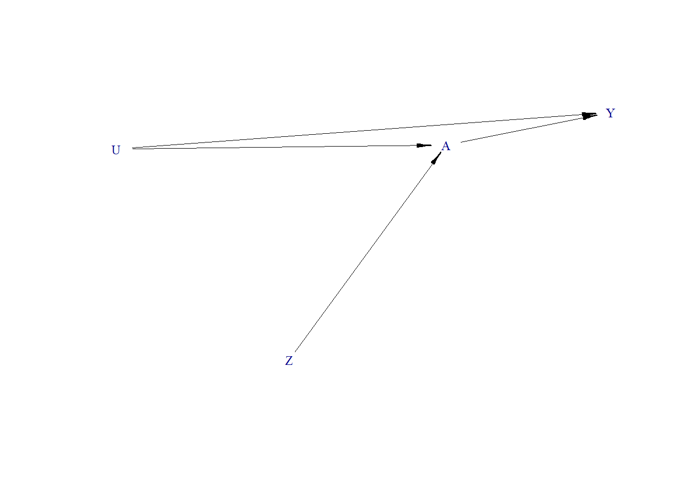
• U is unmeasured continuous variable
• Z is an instrumental variable
• A is binary treatment
• Y is continuous outcome

Non-null effect

• True treatment effect = 1.3

Data generating process

require(simcausal)
D <- DAG.empty()
D <- D + 
  node("U", distr = "rnorm", mean = 2, sd = 1) + 
  node("Z", distr = "rnorm", mean = 2, sd = 1) + 
  node("A", distr = "rbern", prob = plogis(-1 + 2*U + 2*Z)) +
  node("Y", distr = "rnorm", mean = -1 + 3 * U + 1.3 * A, sd = 0.1)
Dset <- set.DAG(D)

Generate DAG

plotDAG(Dset, xjitter = 0.1, yjitter = .9,
        edge_attrs = list(width = 0.5, arrow.width = 0.4, arrow.size = 0.7),
        vertex_attrs = list(size = 12, label.cex = 0.8))

Generate Data

require(simcausal)
Obs.Data <- sim(DAG = Dset, n = 1000000, rndseed = 123)
head(Obs.Data)

ABCDEFGHIJ0123456789

	ID <int>	U <dbl>	Z <dbl>	A <int>	Y <dbl>
1	1	1.439524	0.9919293	1	4.667744
2	2	1.769823	3.3549394	1	5.491603
3	3	3.558708	1.5310251	1	11.063519
4	4	2.070508	3.4681936	1	6.501764
5	5	2.129288	2.4425564	1	6.834678
6	6	3.715065	2.1462031	1	11.340150

6 rows

Estimate effect

# True data generating mechanism (unattainable as U is unmeasured)
fit0 <- glm(Y ~ A + U, family="gaussian", data=Obs.Data)
round(coef(fit0),2)
#> (Intercept)           A           U 
#>        -1.0         1.3         3.0

# Unadjusted effect (Z not controlled)
fit1 <- glm(Y ~ A, family="gaussian", data=Obs.Data)
round(coef(fit1),2)
#> (Intercept)           A 
#>        0.79        5.59

# Bias fit 1
coef(fit1)["A"] - 1.3
#>      A 
#> 4.2935

# Adjusted effect (Z  controlled)
fit2 <- glm(Y ~ A + Z, family="gaussian", data=Obs.Data)
round(coef(fit2),2)
#> (Intercept)           A           Z 
#>        0.86        5.77       -0.12

# Bias from fit 2
coef(fit2)["A"] - 1.3
#>        A 
#> 4.465787

Binary Y

• U is unmeasured continuous variable
• Z is an instrumental variable
• A is binary treatment
• Y is binary outcome

Non-null effect

• True treatment effect = 1.3

Data generating process

require(simcausal)
D <- DAG.empty()
D <- D + 
  node("U", distr = "rnorm", mean = 2, sd = 1) + 
  node("Z", distr = "rnorm", mean = 2, sd = 1) + 
  node("A", distr = "rbern", prob = plogis(-1 + 2*U + 2*Z)) +
  node("Y", distr = "rbern", prob = plogis(-1 + 3 * U + 1.3 * A))
Dset <- set.DAG(D)

Generate DAG

plotDAG(Dset, xjitter = 0.1, yjitter = .9,
        edge_attrs = list(width = 0.5, arrow.width = 0.4, arrow.size = 0.7),
        vertex_attrs = list(size = 12, label.cex = 0.8))

Generate Data

require(simcausal)
Obs.Data <- sim(DAG = Dset, n = 1000000, rndseed = 123)
head(Obs.Data)

ABCDEFGHIJ0123456789

	ID <int>	U <dbl>	Z <dbl>	A <int>	Y <int>
1	1	1.439524	0.9919293	1	1
2	2	1.769823	3.3549394	1	1
3	3	3.558708	1.5310251	1	1
4	4	2.070508	3.4681936	1	1
5	5	2.129288	2.4425564	1	1
6	6	3.715065	2.1462031	1	1

6 rows

Estimate effect

# True data generating mechanism (unattainable as U is unmeasured)
fit0 <- glm(Y ~ A + U, family="binomial", data=Obs.Data)
round(coef(fit0),2)
#> (Intercept)           A           U 
#>       -0.99        1.30        3.01

# Unadjusted effect (Z not controlled)
fit1 <- glm(Y ~ A, family="binomial", data=Obs.Data)
round(coef(fit1),2)
#> (Intercept)           A 
#>        0.40        3.02

# Bias fit 1
coef(fit1)["A"] - 1.3
#>        A 
#> 1.716482

# Adjusted effect (Z  controlled)
fit2 <- glm(Y ~ A + Z, family="binomial", data=Obs.Data)
round(coef(fit2),2)
#> (Intercept)           A           Z 
#>        0.51        3.29       -0.18

# Bias from fit 2
coef(fit2)["A"] - 1.3
#>        A 
#> 1.991396