Mediation Example
We want to decompose of the “total effect” of a given exposure OA (\(A\)) on the outcome CVD (\(Y\)) into
- a natural direct effect (NDE; \(A \rightarrow Y\)) and
- a natural indirect effect (NIE) through a mediator pain medication (\(M\)) through (\(A \rightarrow M \rightarrow Y\)).
Step 0: Build data first
load("Data/mediation/cchs123pain.RData")
source("Data/mediation/medFunc.R")
ls()
#> [1] "analytic.cc"        "analytic.miss"      "doEffectDecomp"
#> [4] "doEffectDecomp.int"

varlist <- c("age", "sex", "income", "race", "bmi", "edu", "phyact", "smoke", "fruit", "diab")
analytic.miss$mediator <- ifelse(analytic.miss$painmed == "Yes", 1, 0)
analytic.miss$exposure <- ifelse(analytic.miss$OA == "OA", 1, 0)
analytic.miss$outcome <- ifelse(analytic.miss$CVD == "event", 1, 0)
Pre-run step 3 model
We will utilize this fit in step 3
# A = actual exposure (without any change)
analytic.miss$exposureTemp <- analytic.miss$exposure

# Design
w.design0 <- svydesign(id=~1, weights=~weight, data=analytic.miss)
w.design <- subset(w.design0, miss == 0)

# Replace exposure with exposureTemp. This will be necessary in step 3
fit.m <- svyglm(mediator ~ exposureTemp +
                 age + sex + income + race + bmi + edu + phyact + smoke + fruit + diab,
                design = w.design, family = binomial("logit"))
#> Warning in eval(family$initialize): non-integer #successes in a binomial glm!
publish(fit.m)
#>      Variable             Units OddsRatio       CI.95     p-value
#>  exposureTemp                        2.43 [2.06;2.86]     < 1e-04
#>           age       20-29 years       Ref
#>                     30-39 years      1.00 [0.88;1.13]   0.9442989
#>                     40-49 years      0.93 [0.82;1.06]   0.2651302
#>                     50-59 years      0.66 [0.58;0.76]     < 1e-04
#>                     60-64 years      0.61 [0.51;0.72]     < 1e-04
#>               65 years and over      0.61 [0.52;0.71]     < 1e-04
#>           sex            Female       Ref
#>                            Male      0.50 [0.46;0.55]     < 1e-04
#>        income   $29,999 or less       Ref
#>                 $30,000-$49,999      1.20 [1.06;1.35]   0.0043533
#>                 $50,000-$79,999      1.21 [1.08;1.37]   0.0014914
#>                 $80,000 or more      1.28 [1.14;1.45]     < 1e-04
#>          race         Non-white       Ref
#>                           White      1.81 [1.62;2.02]     < 1e-04
#>           bmi       Underweight       Ref
#>                  healthy weight      1.09 [0.82;1.44]   0.5631582
#>                      Overweight      1.33 [1.01;1.77]   0.0449616
#>           edu          < 2ndary       Ref
#>                       2nd grad.      1.13 [0.98;1.30]   0.1014986
#>                 Other 2nd grad.      1.30 [1.08;1.55]   0.0050596
#>                  Post-2nd grad.      1.25 [1.10;1.42]   0.0008252
#>        phyact            Active       Ref
#>                        Inactive      1.12 [1.02;1.23]   0.0184447
#>                        Moderate      1.12 [1.01;1.25]   0.0364592
#>         smoke      Never smoker       Ref
#>                  Current smoker      1.29 [1.16;1.44]     < 1e-04
#>                   Former smoker      1.28 [1.17;1.40]     < 1e-04
#>         fruit 0-3 daily serving       Ref
#>               4-6 daily serving      0.92 [0.83;1.02]   0.0976967
#>                6+ daily serving      0.80 [0.71;0.90]   0.0001979
#>          diab                No       Ref
#>                             Yes      1.23 [0.99;1.52]   0.0626501
Step 1 and 2: Replicate data with different exposures
We manipulate and duplicate data here
dim(analytic.miss)
#> [1] 397173     28
dim(analytic.cc)
#> [1] 28734    23
nrow(analytic.miss) - nrow(analytic.cc)
#> [1] 368439

# Create counterfactual data. This will be necessary in step 3
d1 <- d2 <- analytic.miss

# Exposed = Exposed
d1$exposure.counterfactual <- d1$exposure

# Exposed = Not exposed
d2$exposure.counterfactual <- 1 - d2$exposure

# duplicated data (double the amount)
newd <- rbind(d1, d2)
newd <- newd[order(newd$ID), ]
dim(newd)
#> [1] 794346     29
Step 3: Compute weights for the mediation
Weight is computed by
\(W^{M|C} = \frac{P(M|A^*, C)}{P(M|A, C)}\)
in all data newd (fact d1 + alternative fact d2).
-
\(P(M|A, C)\) is computed from a logistic regression of \(M\) on \(A\) + \(C\).
- \(logit [P(M=1 | C = c)] = \beta_0 + \beta_1 a + \beta_3 c\)
-
\(P(M|A^{*}, C)\) is computed from a logistic regression of \(M\) on \(A^*\) + \(C\).
- \(logit [P(M=1 | C = c)] = \beta_0 + \beta'_1 a^* + \beta'_3 c\)
# First, use original exposure (all A + all A):
# A = actual exposure (without any change)
# A = exposure
newd$exposureTemp <- newd$exposure

# Probability of M given A + C
w <- predict(fit.m, newdata=newd, type='response')
direct <- ifelse(newd$mediator, w, 1-w)

# Second, use counterfactual exposures (all A + all !A):
# A* = Opposite (counterfactual) values of the exposure
# A* = exposure.counterfactual
newd$exposureTemp <- newd$exposure.counterfactual

# Probability of M given A* + C
w <- predict(fit.m, newdata=newd, type='response')
indirect <- ifelse(newd$mediator, w, 1-w)

# Mediator weights
newd$W.mediator <- indirect/direct
summary(newd$W.mediator)
#>    Min. 1st Qu.  Median    Mean 3rd Qu.    Max.    NA's
#>    0.45    1.00    1.00    1.01    1.15    2.25  670758
hist(newd$W.mediator)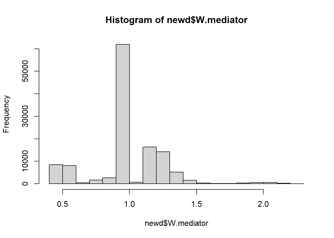
Incorporating the survey weights:
Note: scaling can often be helpful if there exists extreme weights.
# scale survey weights
#newd$S.w <- with(newd,(weight)/mean(weight))
newd$S.w <- with(newd,weight)
newd$S.w[is.na(newd$S.w)]
#> numeric(0)
summary(newd$S.w)
#>    Min. 1st Qu.  Median    Mean 3rd Qu.    Max.
#>    0.39   21.76   42.21   66.70   81.07 2384.98

# Multiply mediator weights with scaled survey weights
newd$SM.w <- with(newd,(W.mediator * S.w))

summary(newd$SM.w)
#>    Min. 1st Qu.  Median    Mean 3rd Qu.    Max.    NA's
#>    0.40   24.65   46.41   73.92   88.84 3531.63  670758
table(newd$miss[is.na(newd$SM.w)])
#>
#>      1
#> 670758
newd$SM.w[is.na(newd$SM.w)] <- 0
summary(newd$SM.w)
#>    Min. 1st Qu.  Median    Mean 3rd Qu.    Max.
#>     0.0     0.0     0.0    11.5     0.0  3531.6

hist(newd$SM.w, main = "", xlab = "Combined weights",
     ylab = "Frequency", freq = TRUE)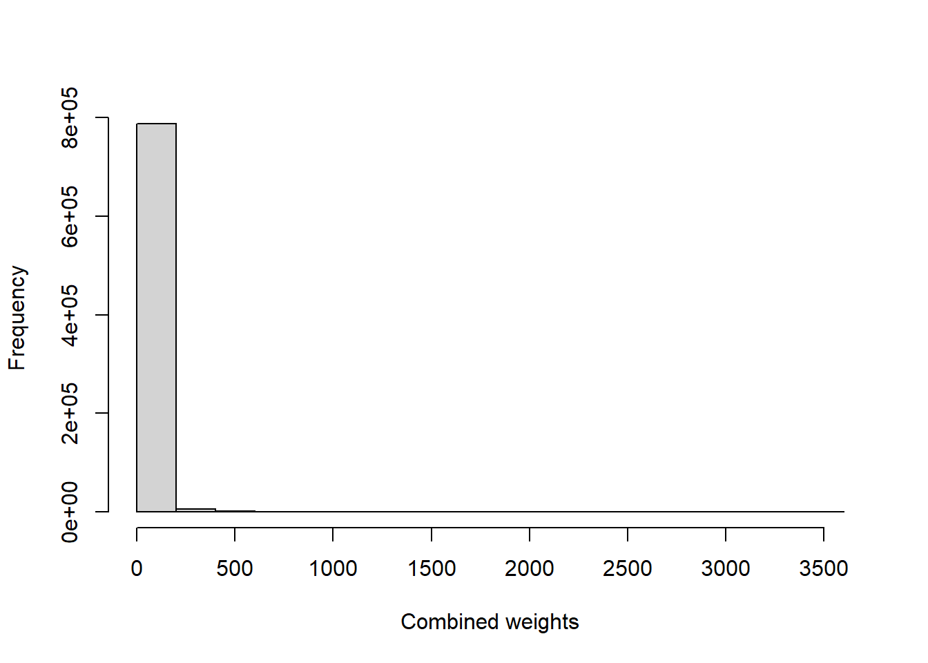
Here all missing weights are associated with incomplete cases (miss==1)! Hence, doesn’t matter if they are missing or other value (0) in them.
Step 4: Weighted outcome Model
Outcome model is
\(logit [P(Y_{a,M(a^*)}=1 | C = c)] = \theta_0 + \theta_1 a + \theta_2 a^* + \theta_3 c\)
after weighting (combination of mediator weight + sampling weight).
# Outcome analysis
w.design0 <- svydesign(id=~1, weights=~SM.w, data=newd)
w.design <- subset(w.design0, miss == 0)

# Fit Y on (A + A* + C)
fit <- svyglm(outcome ~ exposure + exposure.counterfactual +
                age + sex + income + race + bmi + edu + phyact + smoke + fruit + diab,
             design = w.design, family = binomial("logit"))
#> Warning in eval(family$initialize): non-integer #successes in a binomial glm!
Point estimates
Following are the conditional ORs:
- \(OR_{TE}(C=c) = \exp(\theta_1 + \theta_2)\)
- \(OR_{NDE}(A=1,C=c) = \exp(\theta_1)\)
- \(OR_{NIE}(A^{*}=1,C=c) = \exp(\theta_2)\)
These are natural direct and indirect effects (the mediator is not fixed at any value; its distribution is shifted via the weights). They are not controlled effects, which would fix \(M\) at a specific value such as \(M=0\).
# total effect of A-> Y + A -> M -> Y
TE <- exp(sum(coef(fit)[c('exposure', 'exposure.counterfactual')]))
TE
#> [1] 1.544694

# direct effect of A-> Y (not through M)
DE <- exp(unname(coef(fit)['exposure']))
DE
#> [1] 1.488554

# indirect effect of A-> Y (A -> M -> Y)
IE <- exp(unname(coef(fit)[c('exposure.counterfactual')]))
IE
#> [1] 1.037714

# Product of ORs; same as TE
DE * IE
#> [1] 1.544694

# Proportion mediated
PM <- log(IE) / log(TE)
PM
#> [1] 0.08513902
Obtaining results fast
User-written function doEffectDecomp() (specific to OA-CVD problem):
Confidence intervals
Standard errors and confidence intervals are determined by bootstrap methods.
require(boot)
#> Loading required package: boot
#>
#> Attaching package: 'boot'
#> The following object is masked from 'package:survival':
#>
#>     aml
# I ran the computation on a 24 core computer,
# hence set ncpus = 5 (keep some free).
# If you have more / less cores, adjust accordingly.
# Try parallel package to find how many cores you have.
# library(parallel)
# detectCores()
# doEffectDecomp is a user-written function
# See appendix for the function
set.seed(504)
bootresBin <- boot(data=analytic.miss, statistic=doEffectDecomp,
                R = 5, parallel = "multicore", ncpus=5,
                varlist = varlist)
R = 5 is not reliable for bootstrap. In real applications, try 250 at least.
bootci1b <- boot.ci(bootresBin,type = "perc",index=1)
#> Warning in norm.inter(t, alpha): extreme order statistics used as endpoints
bootci2b <- boot.ci(bootresBin,type = "perc",index=2)
#> Warning in norm.inter(t, alpha): extreme order statistics used as endpoints
bootci3b <- boot.ci(bootresBin,type = "perc",index=3)
#> Warning in norm.inter(t, alpha): extreme order statistics used as endpoints
bootci4b <- boot.ci(bootresBin,type = "perc",index=4)
#> Warning in norm.inter(t, alpha): extreme order statistics used as endpoints
# Number of bootstraps
bootresBin$R
#> [1] 5
# Total Effect
c(bootresBin$t0[1], bootci1b$percent[4:5])
#> TE
#> 1.544694 1.293208 1.894417
# Direct Effect
c(bootresBin$t0[2], bootci2b$percent[4:5])
#> DE
#> 1.488554 1.303554 1.876916
# Indirect Effect
c(bootresBin$t0[3], bootci3b$percent[4:5])
#> IE
#> 1.0377144 0.9738072 1.0093246
# Proportion Mediated
c(bootresBin$t0[4], bootci4b$percent[4:5])
#> PM
#> 0.08513902 -0.08360848 0.01655013The proportion mediated through pain medication was about 8.51% on the log odds ratio scale.
Visualization for main effects
require(plotrix)
#> Loading required package: plotrix
TEc <- c(bootresBin$t0[1], bootci1b$percent[4:5])
DEc <- c(bootresBin$t0[2], bootci2b$percent[4:5])
IEc <- c(bootresBin$t0[3], bootci3b$percent[4:5])
mat <- rbind(TEc,DEc,IEc)
colnames(mat) <- c("Point", "2.5%", "97.5%")
mat
#>        Point      2.5%    97.5%
#> TEc 1.544694 1.2932078 1.894417
#> DEc 1.488554 1.3035540 1.876916
#> IEc 1.037714 0.9738072 1.009325

plotCI(1:3, mat[,1], ui=mat[,3], li=mat[,2], xlab = "Estimates", ylab = "", xaxt="n")
axis(1, at=1:3,labels=c("TE","NDE","NIE"))
abline(h=1, lty = 2)
Non-linearity
Consider
- non-linear relationships (polynomials) and interactions between exposure, demographic/baseline covariates and mediators,
- Is misclassification of the mediators possible?
Here we are again using a user-written function doEffectDecomp.int() (including interaction phyact*diab in the mediation model as well as the outcome model):
Visualization for main + interactions
R = 5 is not reliable for bootstrap. In real applications, try 250 at least.
bootci1i <- boot.ci(bootresInt,type = "perc",index=1)
#> Warning in norm.inter(t, alpha): extreme order statistics used as endpoints
bootci2i <- boot.ci(bootresInt,type = "perc",index=2)
#> Warning in norm.inter(t, alpha): extreme order statistics used as endpoints
bootci3i <- boot.ci(bootresInt,type = "perc",index=3)
#> Warning in norm.inter(t, alpha): extreme order statistics used as endpoints
bootci4i <- boot.ci(bootresInt,type = "perc",index=4)
#> Warning in norm.inter(t, alpha): extreme order statistics used as endpointsbootresInt$R
#> [1] 5
# from saved boostrap results: bootresInt
# (similar as before)
TEc <- c(bootresInt$t0[1], bootci1i$percent[4:5])
DEc <- c(bootresInt$t0[2], bootci2i$percent[4:5])
IEc <- c(bootresInt$t0[3], bootci3i$percent[4:5])
mat<- rbind(TEc,DEc,IEc)
colnames(mat) <- c("Point", "2.5%", "97.5%")
mat
#> Point 2.5% 97.5%
#> TEc 1.544720 1.2931358 1.893575
#> DEc 1.488689 1.3040953 1.876521
#> IEc 1.037638 0.9742042 1.009088
plotCI(1:3, mat[,1], ui=mat[,3], li=mat[,2],
xlab = "Estimates", ylab = "", xaxt="n")
axis(1, at=1:3,labels=c("TE","NDE","NIE"))
abline(h=1, lty = 2)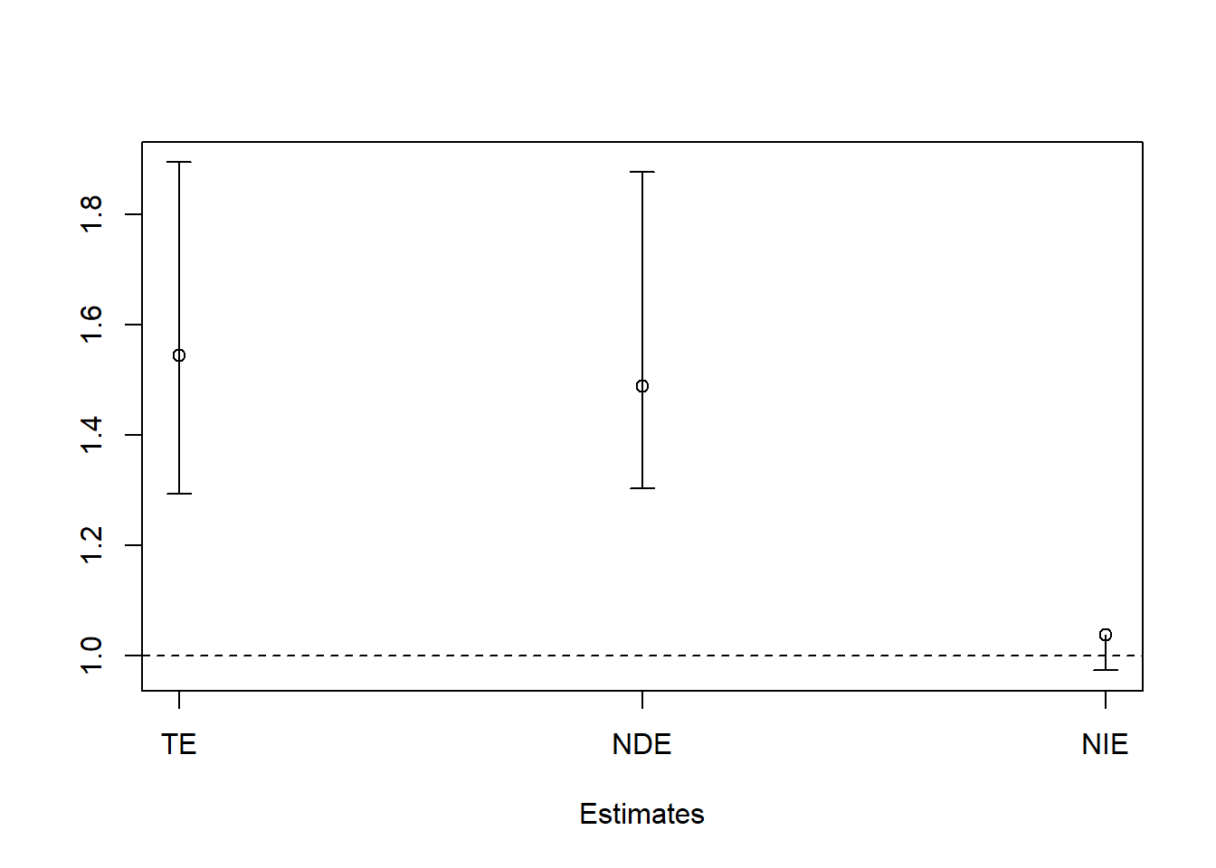
Appendix: OA-CVD Functions for bootstrap
These functions are written basically for performing bootstrap for the OA-CVD analysis. However, changing the covariates names/model-specifications should not be too hard, once you understand the basic steps.
# without interactions (binary mediator)
doEffectDecomp
#> function (dat, ind = NULL, varlist)
#> {
#>     if (is.null(ind))
#>         ind <- 1:nrow(dat)
#>     d <- dat[ind, ]
#>     d$mediator <- ifelse(as.character(d$painmed) == "Yes", 1,
#>         0)
#>     d$exposure <- ifelse(as.character(d$OA) == "OA", 1, 0)
#>     d$outcome <- ifelse(as.character(d$CVD) == "event", 1, 0)
#>     d$exposureTemp <- d$exposure
#>     w.design0 <- svydesign(id = ~1, weights = ~weight, data = d)
#>     w.design <- subset(w.design0, miss == 0)
#>     fit.m <- svyglm(as.formula(paste0(paste0("mediator ~ exposureTemp  + "),
#>         paste0(varlist, collapse = "+"))), design = w.design,
#>         family = quasibinomial("logit"))
#>     d1 <- d2 <- d
#>     d1$exposure.counterfactual <- d1$exposure
#>     d2$exposure.counterfactual <- !d2$exposure
#>     newd <- rbind(d1, d2)
#>     newd <- newd[order(newd$ID), ]
#>     newd$exposureTemp <- newd$exposure
#>     w <- predict(fit.m, newdata = newd, type = "response")
#>     direct <- ifelse(newd$mediator, w, 1 - w)
#>     newd$exposureTemp <- newd$exposure.counterfactual
#>     w <- predict(fit.m, newdata = newd, type = "response")
#>     indirect <- ifelse(newd$mediator, w, 1 - w)
#>     newd$W.mediator <- indirect/direct
#>     summary(newd$W.mediator)
#>     newd$S.w <- with(newd, weight)
#>     summary(newd$S.w)
#>     newd$SM.w <- with(newd, (W.mediator * S.w))
#>     newd$SM.w[is.na(newd$SM.w)] <- 0
#>     summary(newd$SM.w)
#>     w.design0 <- svydesign(id = ~1, weights = ~SM.w, data = newd)
#>     w.design <- subset(w.design0, miss == 0)
#>     fit <- svyglm(as.formula(paste0(paste0("outcome ~ exposure + exposure.counterfactual +"),
#>         paste0(varlist, collapse = "+"))), design = w.design,
#>         family = quasibinomial("logit"))
#>     TE <- exp(sum(coef(fit)[c("exposure", "exposure.counterfactual")]))
#>     DE <- exp(unname(coef(fit)["exposure"]))
#>     IE <- exp(unname(coef(fit)[c("exposure.counterfactual")]))
#>     PM <- log(IE)/log(TE)
#>     return(c(TE = TE, DE = DE, IE = IE, PM = PM))
#> }
#> <bytecode: 0x0000022e10416e10>

# with interactions (binary mediator)
doEffectDecomp.int
#> function (dat, ind = NULL, varlist)
#> {
#>     if (is.null(ind))
#>         ind <- 1:nrow(dat)
#>     d <- dat[ind, ]
#>     d$exposureTemp <- d$exposure
#>     w.design0 <- svydesign(id = ~1, weights = ~weight, data = d)
#>     w.design <- subset(w.design0, miss == 0)
#>     fit.m <- svyglm(as.formula(paste0(paste0("mediator ~ exposureTemp + phyact*diab +"),
#>         paste0(varlist, collapse = "+"))), design = w.design,
#>         family = quasibinomial("logit"))
#>     d1 <- d2 <- d
#>     d1$exposure.counterfactual <- d1$exposure
#>     d2$exposure.counterfactual <- !d2$exposure
#>     newd <- rbind(d1, d2)
#>     newd <- newd[order(newd$ID), ]
#>     newd$exposureTemp <- newd$exposure
#>     w <- predict(fit.m, newdata = newd, type = "response")
#>     direct <- ifelse(newd$mediator, w, 1 - w)
#>     newd$exposureTemp <- newd$exposure.counterfactual
#>     w <- predict(fit.m, newdata = newd, type = "response")
#>     indirect <- ifelse(newd$mediator, w, 1 - w)
#>     newd$W.mediator <- indirect/direct
#>     summary(newd$W.mediator)
#>     newd$S.w <- with(newd, weight)
#>     summary(newd$S.w)
#>     newd$SM.w <- with(newd, (W.mediator * S.w))
#>     newd$SM.w[is.na(newd$SM.w)] <- 0
#>     summary(newd$SM.w)
#>     w.design0 <- svydesign(id = ~1, weights = ~SM.w, data = newd)
#>     w.design <- subset(w.design0, miss == 0)
#>     fit <- svyglm(as.formula(paste0(paste0("outcome ~ exposure + exposure.counterfactual +"),
#>         paste0(varlist, collapse = "+"))), design = w.design,
#>         family = quasibinomial("logit"))
#>     TE <- exp(sum(coef(fit)[c("exposure", "exposure.counterfactual")]))
#>     DE <- exp(unname(coef(fit)["exposure"]))
#>     IE <- exp(unname(coef(fit)[c("exposure.counterfactual")]))
#>     PM <- log(IE)/log(TE)
#>     return(c(TE = TE, DE = DE, IE = IE, PM = PM))
#> }
#> <bytecode: 0x0000022ec5e867f0>
Video content (optional)
For those who prefer a video walkthrough, feel free to watch the video below, which offers a description of an earlier version of the above content.