NHANES: Performance

This tutorial outlines how to evaluate the performance of a logistic regression model fitted to complex survey data using R, focusing on the NHANES dataset.

We will assess the model’s predictive accuracy using a design-correct Area Under the Curve (AUC) and evaluate its fit with the Archer-Lemeshow test.

---

1. Data Preparation ⚙️

First, we need to load the necessary R packages and prepare the NHANES data. The code below loads data from the Flegal2016.RData file, recodes variables like age, race, smoking, and education, and creates the final survey design object (analytic_design) for our analysis.

# --- Load Libraries ---
library(survey)
library(dplyr)
# install.packages("devtools")
# devtools::install_github("ehsanx/svyTable1", 
#                          build_vignettes = TRUE, 
#                          dependencies = TRUE)
library(svyTable1)
library(ggplot2)

# --- Load Data ---
load("Data/surveydata/Flegal2016.RData") 

# --- Create Analytic Sample (N=5,455) ---
dat.analytic <- subset(dat.full, RIDAGEYR >= 20)
dat.analytic <- subset(dat.analytic, !is.na(BMXBMI))
dat.analytic <- subset(dat.analytic, is.na(RIDEXPRG) | RIDEXPRG != "Yes, positive lab pregnancy test")

# --- Recode Analysis Variables ---
dat.full <- dat.full %>%
  mutate(
    Age = cut(RIDAGEYR,
              breaks = c(20, 40, 60, Inf),
              right = FALSE,
              labels = c("20-39", "40-59", ">=60")),

    race = case_when(
      RIDRETH3 == "Non-Hispanic White" ~ "Non-Hispanic white",
      RIDRETH3 == "Non-Hispanic Black" ~ "Non-Hispanic black",
      RIDRETH3 == "Non-Hispanic Asian" ~ "Non-Hispanic Asian",
      RIDRETH3 %in% c("Mexican American", "Other Hispanic") ~ "Hispanic",
      TRUE ~ "Other" # Consolidating "Other Race" for simplicity
    ),
    race = factor(race, levels = c("Non-Hispanic white", "Non-Hispanic black", "Non-Hispanic Asian", "Hispanic", "Other")),

    obese = factor(ifelse(BMXBMI >= 30, "Yes", "No"), levels = c("No", "Yes")),

    smoking = case_when(
      SMQ020 == "No" ~ "Never smoker",
      SMQ020 == "Yes" & SMQ040 == "Not at all" ~ "Former smoker",
      SMQ020 == "Yes" ~ "Current smoker",
      TRUE ~ NA_character_
    ),
    smoking = factor(smoking, levels = c("Never smoker", "Former smoker", "Current smoker")),

    education = case_when(
        DMDEDUC2 %in% c("Less than 9th grade", "9-11th grade (Includes 12th grad)") ~ "<High school",
        DMDEDUC2 == "High school graduate/GED or equi" ~ "High school",
        DMDEDUC2 %in% c("Some college or AA degree", "College graduate or above") ~ ">High school",
        TRUE ~ NA_character_
    ),
    education = factor(education, levels = c("High school", "<High school", ">High school"))
  )

# --- Create Survey Design Object ---
options(survey.lonely.psu = "adjust")
svy.design.full <- svydesign(id = ~SDMVPSU,
                             strata = ~SDMVSTRA,
                             weights = ~WTINT2YR,
                             nest = TRUE,
                             data = dat.full)
analytic_design <- subset(svy.design.full, SEQN %in% dat.analytic$SEQN)

---

2. Fitting a Logistic Regression Model 📊

Next, we fit a survey-weighted logistic regression model using svyglm(). Our goal is to predict obesity status based on Age, race, smoking status, and education level.

# Fit the survey-weighted logistic regression model
fit_obesity <- svyglm(
  I(obese == "Yes") ~ Age + race + smoking + education,
  design = analytic_design,
  family = quasibinomial()
)

---

3. Model Performance: ROC Curve and AUC 📈

We calculate the Area Under the ROC Curve (AUC) to measure predictive performance. The svyAUC() function from svyTable1 computes a design-corrected AUC and confidence interval, which requires a replicate-weights survey design.

Create Replicate Design & Refit Model

# svyAUC() requires a replicate-weights design object
rep_design <- as.svrepdesign(analytic_design)
# Restrict the replicate design to complete cases
vars_for_model <- c("obese", "Age", "race", "smoking", "education")
rep_design_complete <- subset(rep_design, 
                              complete.cases(rep_design$variables[, vars_for_model]))

# Refit model on the complete-case replicate design
fit_obesity_rep <- svyglm(
  I(obese == "Yes") ~ Age + race + smoking + education,
  design = rep_design_complete,
  family = quasibinomial()
)

Calculate AUC

# Calculate the design-correct AUC
auc_results_list <- svyAUC(fit_obesity_rep, rep_design_complete, plot = TRUE)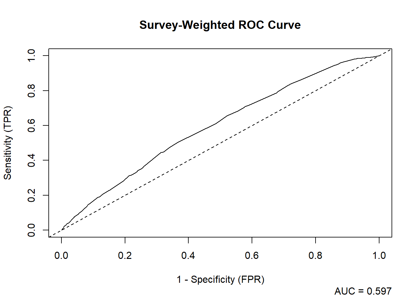

# Display the AUC summary
knitr::kable(auc_results_list$summary)

AUC	SE	CI_Lower	CI_Upper
0.5967987	0.0108604	0.5755123	0.618085

Interpretation: An AUC of 0.5967987 indicates poor discrimination. While better than simpler models, it suggests that the predictors do not have strong predictive power for obesity in this dataset.

Visualize the ROC Curve

ggplot(auc_results_list$roc_data, aes(x = FPR, y = TPR)) +
  geom_line(color = "blue", linewidth = 1) +
  geom_abline(linetype = "dashed") +
  labs(
    title = "Survey-Weighted ROC Curve",
    subtitle = paste0("AUC = ", round(auc_results_list$summary$AUC, 3)),
    x = "1 - Specificity (FPR)",
    y = "Sensitivity (TPR)"
  ) +
  theme_minimal()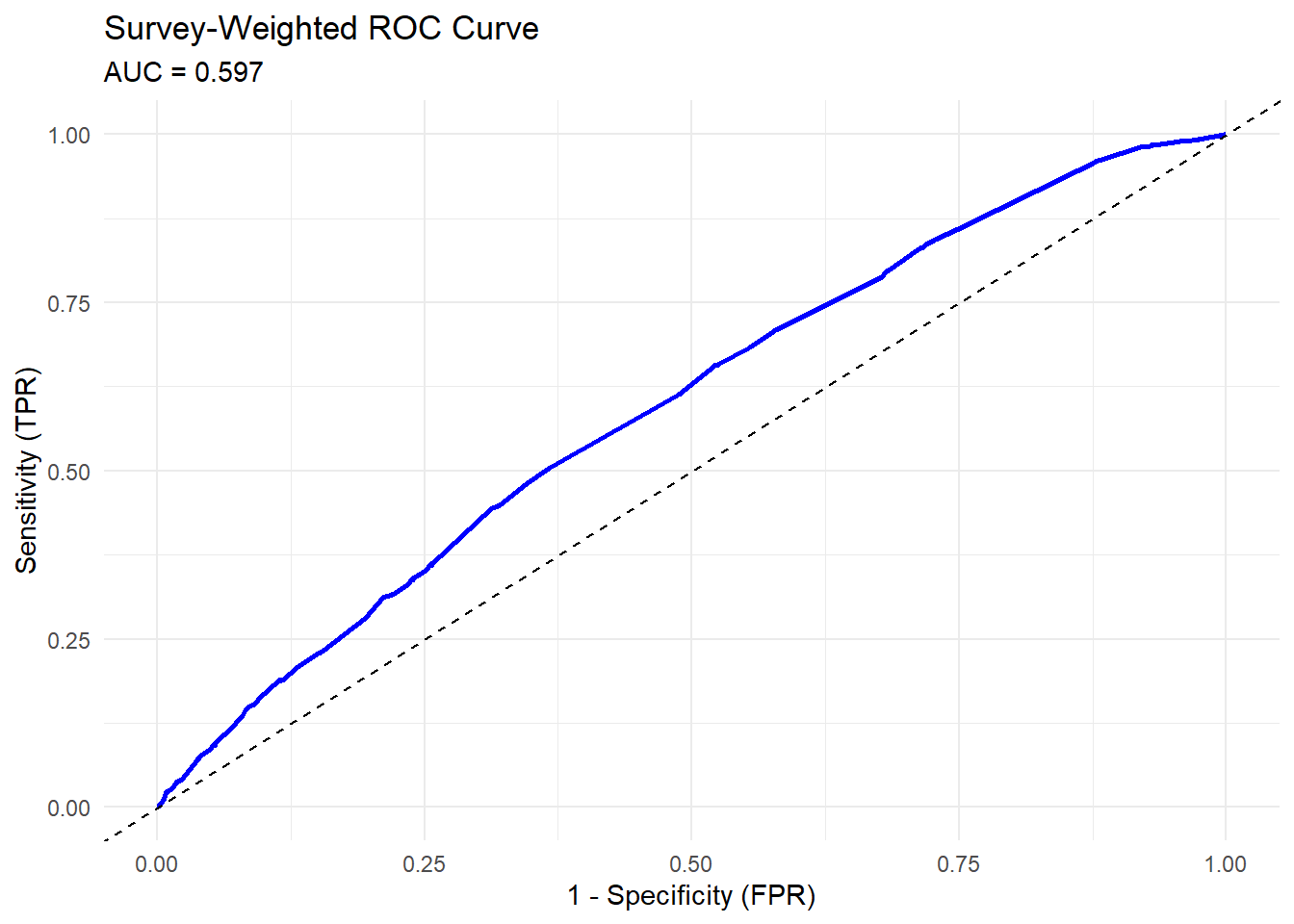

---

4. Goodness-of-Fit: Archer and Lemeshow Test ✅

We assess model fit using the Archer-Lemeshow test. A non-significant p-value (p > 0.05) suggests a good model fit.

# Run the goodness-of-fit test
gof_results <- svygof(fit_obesity, analytic_design)

# Display the results
knitr::kable(gof_results)

F_statistic	df1	df2	p_value
2.168827	9	6	0.1791469

Interpretation: The p-value (0.1791469) is greater than 0.05, indicating no evidence of a poor fit. The model’s predictions align well with observed outcomes, suggesting good calibration.

---

Summary

• The AUC shows poor discriminatory power, meaning the model does not strongly distinguish between obese and non-obese individuals.
• The Archer-Lemeshow test indicates good model fit (p > 0.05).

Conclusion: While well-calibrated, the model’s low predictive power implies other factors (e.g., cholesterol, blood pressure, diet) may better explain obesity risk.