Import external data

# Load required packages
library(dplyr)
require(Hmisc)

When dealing with data analysis in R, it’s common to need to import external data. This tutorial will walk you through importing data in different formats.

CSV format data

CSV stands for “Comma-Separated Values” and it’s a widely used format for data. We’ll be looking at the “Employee Salaries - 2017” dataset, which contains salary information for permanent employees of Montgomery County in 2017.

Employee Salaries - 2017 data

Tip

We’ll be loading the Employee_Salaries_-_2017.csv dataset into R from its saved location at Data/wrangling/. Do note, the directory path might vary for you based on where you’ve stored the downloaded data.

data.download <- read.csv("Data/wrangling/Employee_Salaries_-_2017.csv")

Here, the read.csv function reads the data from the CSV file and stores it in a variable called data.download.

To understand the structure of our dataset, We can see the number of rows and columns and the names of the columns/variables as follows:

dim(data.download) # check dimension / row / column numbers
#> [1] 9398   12
nrow(data.download) # check row numbers
#> [1] 9398
names(data.download) # check column names
#>  [1] "Full.Name"                "Gender"                  
#>  [3] "Current.Annual.Salary"    "X2017.Gross.Pay.Received"
#>  [5] "X2017.Overtime.Pay"       "Department"              
#>  [7] "Department.Name"          "Division"                
#>  [9] "Assignment.Category"      "Employee.Position.Title" 
#> [11] "Position.Under.Filled"    "Date.First.Hired"

Tip

head shows the first 6 elements of an object, giving you a sneak peek into the data you’re dealing with, while tail shows the last 6 elements.

We can see the first see six rows of the dataset as follows:

head(data.download)

Next, for learning purposes, let’s artificially assign all male genders in our dataset as missing:

# Assigning male gender as missing
data.download$Gender[data.download$Gender == "M"] <- NA
head(data.download)

This chunk sets the Gender column’s value to NA (missing) wherever the gender is “M”. This is a form of data manipulation, sometimes used to handle missing or incorrect data. If you want to work with datasets that exclude any missing values:

Tip

na.omit and complete.cases are useful functions to to create datasets with non-NA values

# deleting/dropping missing components
data.download2 <- na.omit(data.download)
head(data.download2)

dim(data.download2)
#> [1] 3806   12

Here, na.omit is used to remove rows with any missing values. This can be essential when preparing data for certain analyses.

Alternatively, we could have selected only females to drop all males:

data.download3 <- filter(data.download, Gender != "M")
head(data.download3)

And to check the size of this new dataset:

# new dimension / row / column numbers
dim(data.download3)
#> [1] 3806   12

SAS format data

Tip

SAS is another data format, commonly used in professional statistics and analytics.

Let’s explore importing a SAS dataset. We download a SAS formatted dataset from the CDC website.

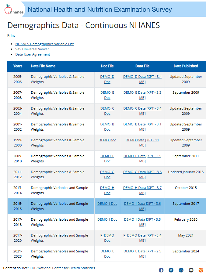
# Link
x <- "https://wwwn.cdc.gov/Nchs/Nhanes/2015-2016/DEMO_I.XPT"

# Data
NHANES1516data <- sasxport.get(x)
#> Processing SAS dataset DEMO_I     ..

# Check dimension / row / column numbers
dim(NHANES1516data) 
#> [1] 9971   47

# Check row numbers
nrow(NHANES1516data) 
#> [1] 9971

# Check first 10 names
names(NHANES1516data)[1:10] 
#>  [1] "seqn"     "sddsrvyr" "ridstatr" "riagendr" "ridageyr" "ridagemn"
#>  [7] "ridreth1" "ridreth3" "ridexmon" "ridexagm"

The sasxport.get function retrieves the SAS dataset. The following lines, just like before, help understand its structure.

To analyze some of the data:

table(NHANES1516data$riagendr) # tabulating gender variable
#> 
#>    1    2 
#> 4892 5079

Verify these numbers from CDC website

This code creates a frequency table of the riagendr variable, which represents gender.