PSM with MI in subset
Problem
In this chapter, we will use propensity score matching (PSM) with multiple imputation, focusing on specific subpopulations defined by the study’s eligibility criteria. We will use PSM as per DuGoff, Schuler, and Stuart (2014) recommendation, with SMD cut-point 0.2 and adjust for imbalanced and/or all covariates in the outcome model, if any.
The modified dataset from NHANES 2017- 2018, which was also used in missing data subpopulations chapter, will be used. This example aims to demonstrate how to do the missing data analysis using multiple imputation with PSM in the context of complex surveys.
Pre-processing
Load data
Let us import the dataset:
Variables
The dataset (dat.full) contains 9,254 subjects with 15 variables:
Survey information
-
studyid: Respondent sequence number -
survey.weight: Full sample 2 year interview weight -
psu: Masked pseudo PSU -
strata: Masked pseudo strata
Outcome variable
-
cvd: Whether having cardiovascular disease
Exposure variable
-
rheumatoid: Whether having rheumatoid arthritis
Covariates
-
age: age in years at screening sexeducation-
race: Race/Ethnicity -
income: Family income in $ -
bmi: Body Mass Index in kg/m\(^2\) -
smoking: Smoking status -
htn: Having hypertension -
diabetes: Having diabetes
Data pre-processng
# Categorical age
dat.full$age.cat <- with(dat.full, ifelse(age >= 20 & age < 50, "20-49",
                                  ifelse(age >= 50 & age < 65, "50-64", "65+")))
dat.full$age.cat <- factor(dat.full$age.cat, levels = c("20-49", "50-64", "65+"))
table(dat.full$age.cat, useNA = "always")
#>
#> 20-49 50-64   65+  <NA>
#>  2500  1569  5185     0

# Recode rheumatoid to arthritis
dat.full$arthritis <- car::recode(dat.full$rheumatoid, " 'No' = 'No arthritis';
                                      'Yes' = 'Rheumatoid arthritis' ", as.factor = T)
table(dat.full$arthritis, useNA = "always")
#>
#>         No arthritis Rheumatoid arthritis                 <NA>
#>                 3857                  337                 5060
Subsetting according to eligibility
We will create the analytic dataset with
- adults aged 20 years or more
- without missing values in outcome (cvd) or exposure (rheumatoid arthritis).
# Drop < 20 years
dat.with.miss <- subset(dat.full, age >= 20)

# Frequency for outcome and exposure
table(dat.with.miss$cvd, useNA = "always") # 6 missing
#>
#>   No  Yes <NA>
#> 4872  691    6
table(dat.with.miss$rheumatoid, useNA = "always") # 1375 missing
#>
#>   No  Yes <NA>
#> 3857  337 1375

# Drop missing in outcome and exposure - dataset with missing values only in covariates
dat.analytic <- dat.with.miss[complete.cases(dat.with.miss$cvd),]
dat.analytic <- dat.analytic[complete.cases(dat.analytic$rheumatoid),]
nrow(dat.analytic)
#> [1] 4191
We have 4,191 participants in our analytic dataset. The general strategy of solution to implement PSM with MI is as follows:
- We will build the imputation model on 4,191 eligible subjects, and
- Apply PSM on each of the imputed datasets, where we will utilize survey features for population-level estimate
- Pool the estimates using Rubin’s rule
variable summary
Let us see the summary statistics as we did in the missing data analysis:
# Keep only relevant variables
vars <-  c("studyid", "survey.weight", "psu", "strata", "cvd", "arthritis", "age.cat",
           "sex", "education", "race", "income", "bmi", "smoking", "htn", "diabetes")
dat.analytic2 <- dat.analytic[, vars]

# Create Table 1
vars <- c("arthritis", "age.cat", "sex", "education", "race", "income", "bmi", "smoking",
          "htn", "diabetes")
tab1 <- CreateTableOne(vars = vars, strata = "cvd", data = dat.analytic2, includeNA = F,
                       addOverall = T, test = F)
print(tab1, format = "f", showAllLevels = T)
#>                  Stratified by cvd
#>                   level                     Overall      No
#>   n                                          4191         3823
#>   arthritis       No arthritis               3854         3580
#>                   Rheumatoid arthritis        337          243
#>   age.cat         20-49                      2280         2240
#>                   50-64                      1097          979
#>                   65+                         814          604
#>   sex             Male                       2126         1884
#>                   Female                     2065         1939
#>   education       Less than high school       828          728
#>                   High school                2292         2094
#>                   College graduate or above  1063          993
#>   race            White                      1275         1113
#>                   Black                       998          898
#>                   Hispanic                   1015          958
#>                   Others                      903          854
#>   income          less than $20,000           659          557
#>                   $20,000 to $74,999         1967         1796
#>                   $75,000 and Over           1143         1079
#>   bmi (mean (SD))                           29.28 (7.19) 29.20 (7.18)
#>   smoking         Never smoker               2570         2427
#>                   Previous smoker             882          726
#>                   Current smoker              739          670
#>   htn             No                         1424         1380
#>                   Yes                        2415         2107
#>   diabetes        No                         3622         3396
#>                   Yes                         566          424
#>                  Stratified by cvd
#>                   Yes
#>   n                 368
#>   arthritis         274
#>                      94
#>   age.cat            40
#>                     118
#>                     210
#>   sex               242
#>                     126
#>   education         100
#>                     198
#>                      70
#>   race              162
#>                     100
#>                      57
#>                      49
#>   income            102
#>                     171
#>                      64
#>   bmi (mean (SD)) 30.09 (7.29)
#>   smoking           143
#>                     156
#>                      69
#>   htn                44
#>                     308
#>   diabetes          226
#>                     142
# missingness
DataExplorer::plot_missing(dat.analytic2)
#> Warning: `aes_string()` was deprecated in ggplot2 3.0.0.
#> ℹ Please use tidy evaluation idioms with `aes()`.
#> ℹ See also `vignette("ggplot2-in-packages")` for more information.
#> ℹ The deprecated feature was likely used in the DataExplorer package.
#> Please report the issue at
#> <https://github.com/boxuancui/DataExplorer/issues>.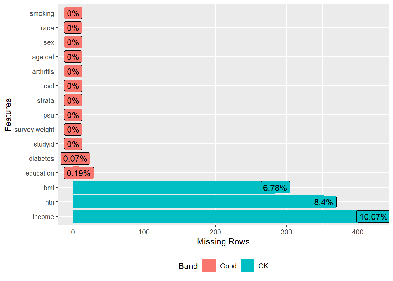
Dealing with missing values in covariates
Similar to the previous exercise, we will create 5 imputed datasets with 3 iterations, and the predictive mean matching method for bmi and income. We will use the strata variable as an auxiliary variable in the imputation model but not the survey weight or PSU variable.
Step 0: Set up the imputation model
# Step 0: Set imputation model
ini <- mice(data = dat.analytic2, maxit = 0, print = FALSE)
pred <- ini$pred

# Use the strata variable as an auxiliary variable in the imputation model
pred["strata",] <- 0

# Do not use survey weight or PSU variable as auxiliary variables
pred[,"studyid"] <- pred["studyid",] <- 0
pred[,"psu"] <- pred["psu",] <- 0
pred[,"survey.weight"] <- pred["survey.weight",] <- 0

# Set imputation method
meth <- ini$meth
meth["bmi"] <- "pmm"
meth["income"] <- "pmm"
meth
#>       studyid survey.weight           psu        strata           cvd
#>            ""            ""            ""            ""            ""
#>     arthritis       age.cat           sex     education          race
#>            ""            ""            ""     "polyreg"            ""
#>        income           bmi       smoking           htn      diabetes
#>         "pmm"         "pmm"            ""      "logreg"      "logreg"
Step 1: Imputing missing values using mice for eligible subjects
Let us save the datasets.
Now we will combine m = 5 datasets and create a stacked dataset. This dataset should contain 5*4,191 = 20,955 rows.
#Remove .id variable from the model as it was created in an intermediate step
impdata$.id <- NULL

# Number of subjects
nrow(impdata)
#> [1] 20955

# Missing after imputation
DataExplorer::plot_missing(impdata)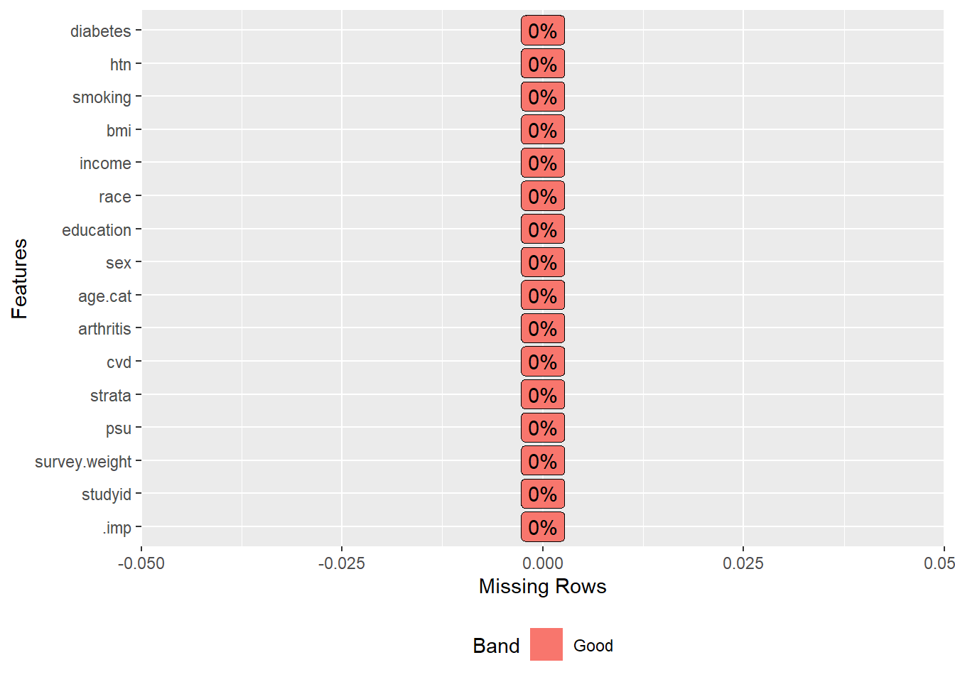
There is no missing value after imputation. There is an additional variable (.imp) in the imputed dataset, which goes from 1 to m = 5, indicating the first to the fifth imputed datasets.
Step 2: PSM steps 1-3 by DuGoff et al. (2014)
Our next step is to use steps 1-3 of the PSM analysis:
- Step 2.1: Fit the PS model by considering survey features as covariates.
- Step 2.2: Match an exposed subject without replacement within the caliper of 0.2 times the standard deviation of the logit of PS.
- Step 2.3: Balance checking using SMD. Consider SMD <0.2 as a good covariate balancing.
Step 2.1: PS model specification
Step 2.2: Estimating PS and matching for each imputed dataset
# Null vector or list to store values
caliper <- NULL
dat.matched <- match.obj <- list(NULL)

m <- 5 # 5 imputed dataset

# PSM on each of the imputed datasets
for (ii in 1:m) {
  # Imputed dataset
  dat.imputed <- subset(impdata, .imp == ii)

  # Propensity scores
  ps.fit <- glm(ps.formula, data = dat.imputed, family = binomial("logit"))
  dat.imputed$ps <- fitted(ps.fit)

  # Caliper fixing to 0.2*sd(logit of PS)
  caliper[ii] <- 0.2*sd(log(dat.imputed$ps/(1-dat.imputed$ps)))

  # 1:1 PS matching
  set.seed(504)
  match.obj[[ii]] <- matchit(ps.formula, data = dat.imputed,
                        distance = dat.imputed$ps,
                        method = "nearest",
                        replace = FALSE,
                        caliper = caliper[ii],
                        ratio = 1)
  dat.imputed$ps <- match.obj[[ii]]$distance

  # Extract matched data
  dat.matched[[ii]] <- match.data(match.obj[[ii]])
}
match.obj
#> [[1]]
#> A `matchit` object
#>  - method: 1:1 nearest neighbor matching without replacement
#>  - distance: User-defined [caliper]
#>  - caliper: <distance> (0.021)
#>  - number of obs.: 4191 (original), 668 (matched)
#>  - target estimand: ATT
#>  - covariates: age.cat, sex, education, race, income, bmi, smoking, htn, diabetes, psu, strata, survey.weight
#>
#> [[2]]
#> A `matchit` object
#>  - method: 1:1 nearest neighbor matching without replacement
#>  - distance: User-defined [caliper]
#>  - caliper: <distance> (0.02)
#>  - number of obs.: 4191 (original), 666 (matched)
#>  - target estimand: ATT
#>  - covariates: age.cat, sex, education, race, income, bmi, smoking, htn, diabetes, psu, strata, survey.weight
#>
#> [[3]]
#> A `matchit` object
#>  - method: 1:1 nearest neighbor matching without replacement
#>  - distance: User-defined [caliper]
#>  - caliper: <distance> (0.021)
#>  - number of obs.: 4191 (original), 672 (matched)
#>  - target estimand: ATT
#>  - covariates: age.cat, sex, education, race, income, bmi, smoking, htn, diabetes, psu, strata, survey.weight
#>
#> [[4]]
#> A `matchit` object
#>  - method: 1:1 nearest neighbor matching without replacement
#>  - distance: User-defined [caliper]
#>  - caliper: <distance> (0.021)
#>  - number of obs.: 4191 (original), 664 (matched)
#>  - target estimand: ATT
#>  - covariates: age.cat, sex, education, race, income, bmi, smoking, htn, diabetes, psu, strata, survey.weight
#>
#> [[5]]
#> A `matchit` object
#>  - method: 1:1 nearest neighbor matching without replacement
#>  - distance: User-defined [caliper]
#>  - caliper: <distance> (0.021)
#>  - number of obs.: 4191 (original), 662 (matched)
#>  - target estimand: ATT
#> - covariates: age.cat, sex, education, race, income, bmi, smoking, htn, diabetes, psu, strata, survey.weightStep 2.3: Balance checking for each imputed dataset
Now we will check balance in terms of SMD on each dataset.
tab1m <- list(NULL)
for (ii in 1:m) {
  # Matched data
  dat <- dat.matched[[ii]]

  # Covariates
  vars <- c("age.cat", "sex", "education", "race", "income", "bmi", "smoking",
            "htn", "diabetes")

  # Balance checking
  tab1m[[ii]] <- CreateTableOne(strata = "arthritis", vars = vars, data = dat, test = F)
}
print(tab1m, smd = TRUE)
#> [[1]]
#>                               Stratified by arthritis
#>                                No arthritis  Rheumatoid arthritis SMD
#>   n                              334           334
#>   age.cat (%)                                                      0.018
#>      20-49                        51 (15.3)     52 (15.6)
#>      50-64                       131 (39.2)    133 (39.8)
#>      65+                         152 (45.5)    149 (44.6)
#>   sex = Female (%)               172 (51.5)    178 (53.3)          0.036
#>   education (%)                                                    0.034
#>      Less than high school        80 (24.0)     84 (25.1)
#>      High school                 204 (61.1)    203 (60.8)
#>      College graduate or above    50 (15.0)     47 (14.1)
#>   race (%)                                                         0.049
#>      White                       105 (31.4)    103 (30.8)
#>      Black                       107 (32.0)    112 (33.5)
#>      Hispanic                     67 (20.1)     69 (20.7)
#>      Others                       55 (16.5)     50 (15.0)
#>   income (%)                                                       0.073
#>      less than $20,000            95 (28.4)    100 (29.9)
#>      $20,000 to $74,999          162 (48.5)    167 (50.0)
#>      $75,000 and Over             77 (23.1)     67 (20.1)
#>   bmi (mean (SD))              30.62 (8.16)  30.54 (7.34)          0.011
#>   smoking (%)                                                      0.052
#>      Never smoker                158 (47.3)    161 (48.2)
#>      Previous smoker             102 (30.5)    106 (31.7)
#>      Current smoker               74 (22.2)     67 (20.1)
#>   htn = Yes (%)                  283 (84.7)    279 (83.5)          0.033
#>   diabetes = Yes (%)             106 (31.7)    100 (29.9)          0.039
#>
#> [[2]]
#>                               Stratified by arthritis
#>                                No arthritis  Rheumatoid arthritis SMD
#>   n                              333           333
#>   age.cat (%)                                                      0.055
#>      20-49                        50 (15.0)     52 (15.6)
#>      50-64                       142 (42.6)    133 (39.9)
#>      65+                         141 (42.3)    148 (44.4)
#>   sex = Female (%)               172 (51.7)    176 (52.9)          0.024
#>   education (%)                                                    0.068
#>      Less than high school        92 (27.6)     84 (25.2)
#>      High school                 191 (57.4)    202 (60.7)
#>      College graduate or above    50 (15.0)     47 (14.1)
#>   race (%)                                                         0.146
#>      White                        91 (27.3)    104 (31.2)
#>      Black                       100 (30.0)    110 (33.0)
#>      Hispanic                     79 (23.7)     69 (20.7)
#>      Others                       63 (18.9)     50 (15.0)
#>   income (%)                                                       0.131
#>      less than $20,000           115 (34.5)     96 (28.8)
#>      $20,000 to $74,999          166 (49.8)    175 (52.6)
#>      $75,000 and Over             52 (15.6)     62 (18.6)
#>   bmi (mean (SD))              30.50 (7.88)  30.51 (7.46)          0.001
#>   smoking (%)                                                      0.015
#>      Never smoker                160 (48.0)    161 (48.3)
#>      Previous smoker             104 (31.2)    105 (31.5)
#>      Current smoker               69 (20.7)     67 (20.1)
#>   htn = Yes (%)                  288 (86.5)    278 (83.5)          0.084
#>   diabetes = Yes (%)              97 (29.1)     99 (29.7)          0.013
#>
#> [[3]]
#>                               Stratified by arthritis
#>                                No arthritis  Rheumatoid arthritis SMD
#>   n                              336           336
#>   age.cat (%)                                                      0.077
#>      20-49                        46 (13.7)     52 (15.5)
#>      50-64                       145 (43.2)    133 (39.6)
#>      65+                         145 (43.2)    151 (44.9)
#>   sex = Female (%)               176 (52.4)    179 (53.3)          0.018
#>   education (%)                                                    0.076
#>      Less than high school        80 (23.8)     86 (25.6)
#>      High school                 215 (64.0)    203 (60.4)
#>      College graduate or above    41 (12.2)     47 (14.0)
#>   race (%)                                                         0.084
#>      White                       114 (33.9)    105 (31.2)
#>      Black                       114 (33.9)    112 (33.3)
#>      Hispanic                     59 (17.6)     69 (20.5)
#>      Others                       49 (14.6)     50 (14.9)
#>   income (%)                                                       0.118
#>      less than $20,000            87 (25.9)    104 (31.0)
#>      $20,000 to $74,999          183 (54.5)    166 (49.4)
#>      $75,000 and Over             66 (19.6)     66 (19.6)
#>   bmi (mean (SD))              30.56 (7.71)  30.54 (7.53)          0.003
#>   smoking (%)                                                      0.127
#>      Never smoker                180 (53.6)    161 (47.9)
#>      Previous smoker              89 (26.5)    107 (31.8)
#>      Current smoker               67 (19.9)     68 (20.2)
#>   htn = Yes (%)                  280 (83.3)    281 (83.6)          0.008
#>   diabetes = Yes (%)             104 (31.0)    102 (30.4)          0.013
#>
#> [[4]]
#>                               Stratified by arthritis
#>                                No arthritis  Rheumatoid arthritis SMD
#>   n                              332           332
#>   age.cat (%)                                                      0.062
#>      20-49                        48 (14.5)     52 (15.7)
#>      50-64                       127 (38.3)    133 (40.1)
#>      65+                         157 (47.3)    147 (44.3)
#>   sex = Female (%)               174 (52.4)    175 (52.7)          0.006
#>   education (%)                                                    0.059
#>      Less than high school        79 (23.8)     85 (25.6)
#>      High school                 200 (60.2)    200 (60.2)
#>      College graduate or above    53 (16.0)     47 (14.2)
#>   race (%)                                                         0.034
#>      White                       100 (30.1)    105 (31.6)
#>      Black                       111 (33.4)    108 (32.5)
#>      Hispanic                     71 (21.4)     69 (20.8)
#>      Others                       50 (15.1)     50 (15.1)
#>   income (%)                                                       0.067
#>      less than $20,000            93 (28.0)     95 (28.6)
#>      $20,000 to $74,999          165 (49.7)    172 (51.8)
#>      $75,000 and Over             74 (22.3)     65 (19.6)
#>   bmi (mean (SD))              30.06 (7.85)  30.46 (7.49)          0.052
#>   smoking (%)                                                      0.053
#>      Never smoker                166 (50.0)    161 (48.5)
#>      Previous smoker              97 (29.2)    105 (31.6)
#>      Current smoker               69 (20.8)     66 (19.9)
#>   htn = Yes (%)                  281 (84.6)    278 (83.7)          0.025
#>   diabetes = Yes (%)              93 (28.0)     98 (29.5)          0.033
#>
#> [[5]]
#>                               Stratified by arthritis
#>                                No arthritis  Rheumatoid arthritis SMD
#>   n                              331           331
#>   age.cat (%)                                                      0.026
#>      20-49                        50 (15.1)     52 (15.7)
#>      50-64                       137 (41.4)    133 (40.2)
#>      65+                         144 (43.5)    146 (44.1)
#>   sex = Female (%)               172 (52.0)    175 (52.9)          0.018
#>   education (%)                                                    0.025
#>      Less than high school        86 (26.0)     84 (25.4)
#>      High school                 196 (59.2)    200 (60.4)
#>      College graduate or above    49 (14.8)     47 (14.2)
#>   race (%)                                                         0.026
#>      White                        99 (29.9)    103 (31.1)
#>      Black                       111 (33.5)    109 (32.9)
#>      Hispanic                     70 (21.1)     69 (20.8)
#>      Others                       51 (15.4)     50 (15.1)
#>   income (%)                                                       0.074
#>      less than $20,000            84 (25.4)     94 (28.4)
#>      $20,000 to $74,999          181 (54.7)    170 (51.4)
#>      $75,000 and Over             66 (19.9)     67 (20.2)
#>   bmi (mean (SD))              30.17 (7.58)  30.49 (7.86)          0.042
#>   smoking (%)                                                      0.027
#>      Never smoker                165 (49.8)    161 (48.6)
#>      Previous smoker             104 (31.4)    105 (31.7)
#>      Current smoker               62 (18.7)     65 (19.6)
#>   htn = Yes (%)                  276 (83.4)    277 (83.7)          0.008
#>   diabetes = Yes (%)             102 (30.8)     97 (29.3)          0.033
For each of the datasets, all SMDs are less than our specified cut-point of 0.2.
Step 3: Outcome modelling
Our next step is to fit the outcome model on each of the imputed dataset. Remember, we must utilize survey features to correctly estimate the standard error.
3.1 Preparing dataset for ineligible subjects
Now we will add the ineligible subjects(ineligible by study restriction and unmatched) with the matched datasets, so that we can set up the survey design on the full dataset and then subset the design.
Let us subset the data for ineligible subjects:
# Subset for ineligible
dat.ineligible <- list(NULL)

for(ii in 1:m){
  # Matched dataset
  dat <- dat.matched[[ii]]

  # Create an indicator variable in the full dataset
  dat.full$ineligible <- 1
  dat.full$ineligible[dat.full$studyid %in% dat$studyid] <- 0

  # Subset for ineligible
  dat.ineligible[[ii]] <- subset(dat.full, ineligible == 1)

  # Create the .imp variable on each dataset with .imp 1 to m = 5
  dat.ineligible[[ii]]$.imp <- ii
}

# Dimension of each dataset
lapply(dat.ineligible, dim)
#> [[1]]
#> [1] 8586   19
#>
#> [[2]]
#> [1] 8588   19
#>
#> [[3]]
#> [1] 8582   19
#>
#> [[4]]
#> [1] 8590   19
#>
#> [[5]]
#> [1] 8592   19
The next step is combining matched and ineligible datasets. Before merging, we must ensure the variable names are the same.
# Variables in the matched datasets
names(dat.matched[[3]])
#>  [1] "studyid"       "survey.weight" "psu"           "strata"
#>  [5] "cvd"           "arthritis"     "age.cat"       "sex"
#>  [9] "education"     "race"          "income"        "bmi"
#> [13] "smoking"       "htn"           "diabetes"      ".imp"
#> [17] "ps"            "distance"      "weights"       "subclass"

# Variables in the ineligible datasets
names(dat.ineligible[[3]])
#>  [1] "studyid"       "survey.weight" "psu"           "strata"
#>  [5] "cvd"           "rheumatoid"    "age"           "sex"
#>  [9] "education"     "race"          "income"        "bmi"
#> [13] "smoking"       "htn"           "diabetes"      "age.cat"
#> [17] "arthritis"     "ineligible"    ".imp"
Four variables (ps, distance, weights, and subclass) are unavailable in our full, analytic, or ineligible datasets but in the matched datasets. We need to create these 4 variables in the ineligible datasets.
dat.ineligible2 <- list(NULL)

for (ii in 1:m) {
  dat <- dat.ineligible[[ii]]

  # Drop the ineligible variable from the dataset
  dat$ineligible <- NULL

  # Create ps, distance, weights, and subclass
  dat$ps <- NA
  dat$distance <- NA
  dat$weights <- NA
  dat$subclass <- NA

  # Keep only those variables available in the matched dataset
  vars <- names(dat.matched[[1]])
  dat <- dat[,vars]

  # Ineligible datasets in list format
  dat.ineligible2[[ii]] <- dat
}
We created ps, distance, weights, and subclass with missing values for the ineligible participants. Note that it doesn’t matter whether there are missing covariate values for ineligible. Since we will create the design on the full dataset and subset the design for only eligible (i.e., matched participants), missing covariate values for ineligible will not impact our analysis.
3.2 Combining eligible (matched) and ineligible (unimputed + unmatched) subjects
Now, we will merge matched eligible and unimputed and unmatched ineligible subjects. We should have m = 5 copies of the full dataset with 9,254 subjects on each.
dat.full2 <- list(NULL)

for (ii in 1:m) {
  # Eligible
  d1 <- data.frame(dat.matched[[ii]])
  d1$eligible <- 1

  # Ineligible
  d2 <- data.frame(dat.ineligible2[[ii]])
  d2$eligible <- 0

  # Full data
  d3 <- rbind(d1, d2)
  dat.full2[[ii]] <- d3
}
lapply(dat.full2, dim)
#> [[1]]
#> [1] 9254   21
#>
#> [[2]]
#> [1] 9254   21
#>
#> [[3]]
#> [1] 9254   21
#>
#> [[4]]
#> [1] 9254   21
#>
#> [[5]]
#> [1] 9254   21

# Stacked dataset
dat.stacked <- rbindlist(dat.full2)
dim(dat.stacked)
#> [1] 46270    21
3.3 Prepating Survey design and subpopulation of eligible
The next step is to create the design on the combined dataset.
allImputations <- imputationList(lapply(1:m, function(n) subset(dat.stacked, subset=.imp==n)))

# Design on full data
w.design0 <- svydesign(ids = ~psu,
                       weights = ~survey.weight,
                       strata = ~strata,
                      data = allImputations,
                      nest = TRUE)

# Subset the design
w.design <- subset(w.design0, eligible == 1)
#> Warning in subset.svyimputationList(w.design0, eligible == 1): subset differed
#> between imputations
We can see the length of the subsetted design:
Now we will run the design-adjusted logistic regression on and pool the estimate using Rubin’s rule:
Step 3.4: Design adjusted regression analysis
# Design-adjusted logistic regression
fit <- with(w.design, svyglm(I(cvd == "Yes") ~ arthritis, family = quasibinomial))
res <- exp(as.data.frame(cbind(coef(fit[[1]]),
                               coef(fit[[2]]),
                               coef(fit[[3]]),
                               coef(fit[[4]]),
                               coef(fit[[5]]))))
names(res) <- paste("OR from m =", 1:m)
round(t(res),2)
#>               (Intercept) arthritisRheumatoid arthritis
#> OR from m = 1        0.18                          1.53
#> OR from m = 2        0.24                          1.09
#> OR from m = 3        0.21                          1.28
#> OR from m = 4        0.17                          1.61
#> OR from m = 5        0.12                          2.32
Step 3.5: Pooling estimates
Double adjustment
# Outcome model with covariates adjustment
fit2 <- with(w.design, svyglm(I(cvd == "Yes") ~ arthritis + age.cat + sex + education +
                               race + income + bmi + smoking + htn + diabetes,
                             family = quasibinomial))

# Pooled estimate
pooled.estimates <- MIcombine(fit2)
OR <- round(exp(pooled.estimates$coefficients), 2)
OR <- as.data.frame(OR)
CI <- round(exp(confint(pooled.estimates)), 2)
OR <- cbind(OR, CI)
OR