Subpopulations

This tutorial demonstrates how to manage missing data in complex surveys using multiple imputation, focusing on specific subpopulations defined by the study’s eligibility criteria.

Purpose

Let us we are interested in exploring the relationship between rheumatoid arthritis and cardiovascular disease (CVD) among US adults aged 20 years or more. For that, we will use NHANES 2017–2018 dataset, which follows a complex survey design.

In this tutorial, we used a similar approach to the one in a published article by Hossain et al. (2022), but we used less data (restricted to only 2017–2018) to speed up the analysis. Ref link.

The purpose of this example is to demonstrate how to do the missing data analysis with multiple imputation in the context of complex surveys.

The main idea is:

working with the analytic data
imputing missing values based on that analytic dataset
keep count of the ineligible subjects from the full data who are not included in the analytic data
adding those ineligible subjects back in the imputed datasets, so that we can utilize the survey features and subset the design.

# Load required packages
library(dplyr)
library(kableExtra)
library(tableone)
library(survey)
library(Publish)
library(DataExplorer)
library(mice)
library(mitools)

Let us import the dataset:

load("Data/missingdata/MIexample.RData")
ls()
#> [1] "dat.full"

dim(dat.full)
#> [1] 9254   15
head(dat.full)

The dataset (dat.full) contains 9,254 subjects with 15 variables:

Survey information

studyid: Respondent sequence number
survey.weight: Full sample 2 year interview weight
psu: Masked pseudo PSU
strata: Masked pseudo strata

Outcome variable

cvd: Whether having cardiovascular disease

Exposure variable

rheumatoid: Whether having rheumatoid arthritis

Covariates

age: age in years at screening
sex
education
race: Race/Ethnicity
income: Family income in $
bmi: Body Mass Index in kg/m$^2$
smoking: Smoking status
htn: Having hypertension
diabetes: Having diabetes

Analytic dataset

Subsetting according to eligibility

Let us create an analytic dataset for

adults aged 20 years or more
without missing values in outcome (cvd) or exposure (rheumatoid arthritis).

# Drop < 20 years
dat.with.miss <- subset(dat.full, age >= 20)

# Frequency for outcome and exposure 
table(dat.with.miss$cvd, useNA = "always") # 6 missing
#> 
#>   No  Yes <NA> 
#> 4872  691    6
table(dat.with.miss$rheumatoid, useNA = "always") # 1375 missing
#> 
#>   No  Yes <NA> 
#> 3857  337 1375

# Drop missing in outcome and exposure 
# i.e., dataset with missing values only in covariates
dat.analytic <- dat.with.miss[complete.cases(dat.with.miss$cvd),]
dat.analytic <- dat.analytic[complete.cases(dat.analytic$rheumatoid),]
nrow(dat.analytic)
#> [1] 4191

As we can see, we have 4,191 participants aged 20 years or more without missing values in outcome or exposure. Let us count the ineligible subjects from the full data and create an indicator variable.

dat.full$ineligible <- 1
dat.full$ineligible[dat.full$studyid %in% dat.analytic$studyid] <- 0
table(dat.full$ineligible, useNA = "always")
#> 
#>    0    1 <NA> 
#> 4191 5063    0

We have 4,191 eligible and 5,063 ineligible subjects based on the eligibility criteria.

General strategy of solution:

We will build the imputation model on 4,191 eligible subjects, and
later we will include 5,063 ineligible subjects in the data so that we can utilize survey features.

Table 1

Let us see the summary statistics, i.e., create Table 1 stratified by outcome (cvd). Before that, we will categorize age and recode rheumatoid:

# Categorical age
dat.analytic$age.cat <- 
  with(dat.analytic, ifelse(age >= 20 & age < 50, "20-49", 
                            ifelse(age >= 50 & age < 65, 
                                   "50-64", "65+")))
dat.analytic$age.cat <- factor(dat.analytic$age.cat, 
                               levels = c("20-49", "50-64", "65+"))
table(dat.analytic$age.cat, useNA = "always")
#> 
#> 20-49 50-64   65+  <NA> 
#>  2280  1097   814     0

# Recode rheumatoid to arthritis
dat.analytic$arthritis <- 
car::recode(dat.analytic$rheumatoid, " 'No' = 'No arthritis';
            'Yes' = 'Rheumatoid arthritis' ", as.factor = T)
table(dat.analytic$arthritis, useNA = "always")
#> 
#>         No arthritis Rheumatoid arthritis                 <NA> 
#>                 3854                  337                    0

# Keep only relevant variables
vars <-  c("studyid", "survey.weight", "psu", "strata", "cvd",
           "arthritis", "age.cat", "sex", "education", "race",
           "income", "bmi", "smoking", "htn", "diabetes")
dat.analytic2 <- dat.analytic[, vars]

# Create Table 1
vars <- c("arthritis", "age.cat", "sex", "education", "race", "income", "bmi", "smoking",
          "htn", "diabetes")
tab1 <- CreateTableOne(vars = vars, strata = "cvd", 
                       data = dat.analytic2, includeNA = F,
                       addOverall = T, test = F)
print(tab1, format = "f", showAllLevels = T)
#>                  Stratified by cvd
#>                   level                     Overall      No          
#>   n                                          4191         3823       
#>   arthritis       No arthritis               3854         3580       
#>                   Rheumatoid arthritis        337          243       
#>   age.cat         20-49                      2280         2240       
#>                   50-64                      1097          979       
#>                   65+                         814          604       
#>   sex             Male                       2126         1884       
#>                   Female                     2065         1939       
#>   education       Less than high school       828          728       
#>                   High school                2292         2094       
#>                   College graduate or above  1063          993       
#>   race            White                      1275         1113       
#>                   Black                       998          898       
#>                   Hispanic                   1015          958       
#>                   Others                      903          854       
#>   income          less than $20,000           659          557       
#>                   $20,000 to $74,999         1967         1796       
#>                   $75,000 and Over           1143         1079       
#>   bmi (mean (SD))                           29.28 (7.19) 29.20 (7.18)
#>   smoking         Never smoker               2570         2427       
#>                   Previous smoker             882          726       
#>                   Current smoker              739          670       
#>   htn             No                         1424         1380       
#>                   Yes                        2415         2107       
#>   diabetes        No                         3622         3396       
#>                   Yes                         566          424       
#>                  Stratified by cvd
#>                   Yes         
#>   n                 368       
#>   arthritis         274       
#>                      94       
#>   age.cat            40       
#>                     118       
#>                     210       
#>   sex               242       
#>                     126       
#>   education         100       
#>                     198       
#>                      70       
#>   race              162       
#>                     100       
#>                      57       
#>                      49       
#>   income            102       
#>                     171       
#>                      64       
#>   bmi (mean (SD)) 30.09 (7.29)
#>   smoking           143       
#>                     156       
#>                      69       
#>   htn                44       
#>                     308       
#>   diabetes          226       
#>                     142

Check missingness using a plot

Now we will see the percentage of missing values in the variables.

DataExplorer::plot_missing(dat.analytic2)

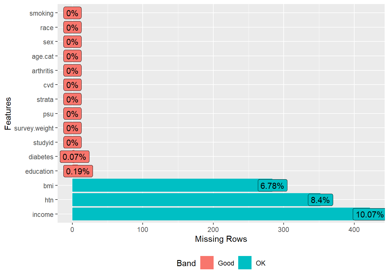
We have about 10% missing values in income, followed by hypertension (8.4%), bmi (6.8%), education (0.2%), and diabetes (0.1%).

Dealing with missing values in covariates

Now we will perform multiple imputation to deal with missing values only in covariates. We will use the dat.analytic2 dataset that contains missing values in the covariates but no missing values in the outcome or exposure.
For this exercise, we will consider 5 imputed datasets, 3 iterations, and the predictive mean matching method for bmi and income.
- We have already set up the data such that the variables are of appropriate types, e.g., numeric bmi, factor age, sex, and so on.
- We will use the strata variable as an auxiliary variable in the imputation model but not the survey weight or PSU variable.
- Now we will set up the initial model and set up the methods and predictor matrix before imputing 5 datasets.

Step 0: Set up the imputation model

In this tutorial, we used stata as an auxiliary variable. There are two ways we can deal with this:

Use strata to predict other variables, but don’t impute strata: meth["strata"] <- "" (this skips strata’s imputation). In our case, since strata has no missing observations, this step is unnecessary, as MICE will automatically not impute fully observed variables. However, this strategy is useful for blocking the imputation of auxiliary variables with missing data.

Also, do not change the predictorMatrix for auxiliary variables, allowing them (e.g., strata in our case) to be used as predictors for other variables.
Setting pred["strata", ] <- 0 would remove all predictors for strata, which means strata cannot be imputed because there are no variables to predict its missing values. However, strata can still be used as a predictor for other variables. If strata has no missing values (as in our case), this step is unnecessary since MICE does not attempt to impute fully observed variables.

Impute strata and use it as a predictor (if strata had missing values): If strata had missing data, you wouldn’t need to change anything in predictorMatrix or method. MICE would impute strata and use it as a predictor by default. In our case, since strata has no missing values, imputation is not necessary. Note that:

You should not set pred["strata", ] <- 1 because this would incorrectly make strata a predictor for itself, which is invalid. MICE automatically handles this by setting diagonal entries to 0, so you don’t need to manually ensure this unless you’ve changed it. If you do so (set the row values to 1), you need to then set pred["strata", "strata"] <- 0 to ensure strata does not predict itself.
Do not use pred[, "strata"] <- 0 because this would prevent strata from being used as a predictor for other variables, which is contrary to the idea of using it as an auxiliary variable.

Whether to impute or not impute auxiliary variables depends on their role in the analysis and the potential impact of their missing data. If they are strong predictors or are necessary for future analyses, imputing them may be justified. However, if their missingness is not consequential, and imputing them introduces more noise or complexity, it may be better to leave them unimputed.

# Step 0: Set imputation model
ini <- mice(data = dat.analytic2, maxit = 0, print = FALSE)
pred <- ini$pred

kable(pred)

	studyid	survey.weight	psu	strata	cvd	arthritis	age.cat	sex	education	race	income	bmi	smoking	htn	diabetes
studyid	0	1	1	1	1	1	1	1	1	1	1	1	1	1	1
survey.weight	1	0	1	1	1	1	1	1	1	1	1	1	1	1	1
psu	1	1	0	1	1	1	1	1	1	1	1	1	1	1	1
strata	1	1	1	0	1	1	1	1	1	1	1	1	1	1	1
cvd	1	1	1	1	0	1	1	1	1	1	1	1	1	1	1
arthritis	1	1	1	1	1	0	1	1	1	1	1	1	1	1	1
age.cat	1	1	1	1	1	1	0	1	1	1	1	1	1	1	1
sex	1	1	1	1	1	1	1	0	1	1	1	1	1	1	1
education	1	1	1	1	1	1	1	1	0	1	1	1	1	1	1
race	1	1	1	1	1	1	1	1	1	0	1	1	1	1	1
income	1	1	1	1	1	1	1	1	1	1	0	1	1	1	1
bmi	1	1	1	1	1	1	1	1	1	1	1	0	1	1	1
smoking	1	1	1	1	1	1	1	1	1	1	1	1	0	1	1
htn	1	1	1	1	1	1	1	1	1	1	1	1	1	0	1
diabetes	1	1	1	1	1	1	1	1	1	1	1	1	1	1	0


# Use the strata variable as an auxiliary variable in the imputation model
pred["strata",]
#>       studyid survey.weight           psu        strata           cvd 
#>             1             1             1             0             1 
#>     arthritis       age.cat           sex     education          race 
#>             1             1             1             1             1 
#>        income           bmi       smoking           htn      diabetes 
#>             1             1             1             1             1
# Do not change the pred matrix for strata. 
# This allows strata to be used as a predictor for other variables.

# Do not use id, survey weight or PSU variable as auxiliary variables
pred[, c("studyid", "psu", "survey.weight")] <- 0
# Remove them as predictors for other variables

kable(pred)

	strata	cvd	arthritis	age.cat	sex	education	race	income	bmi	smoking	htn	diabetes
studyid	1	1	1	1	1	1	1	1	1	1	1	1
survey.weight	1	1	1	1	1	1	1	1	1	1	1	1
psu	1	1	1	1	1	1	1	1	1	1	1	1
strata	0	1	1	1	1	1	1	1	1	1	1	1
cvd	1	0	1	1	1	1	1	1	1	1	1	1
arthritis	1	1	0	1	1	1	1	1	1	1	1	1
age.cat	1	1	1	0	1	1	1	1	1	1	1	1
sex	1	1	1	1	0	1	1	1	1	1	1	1
education	1	1	1	1	1	0	1	1	1	1	1	1
race	1	1	1	1	1	1	0	1	1	1	1	1
income	1	1	1	1	1	1	1	0	1	1	1	1
bmi	1	1	1	1	1	1	1	1	0	1	1	1
smoking	1	1	1	1	1	1	1	1	1	0	1	1
htn	1	1	1	1	1	1	1	1	1	1	0	1
diabetes	1	1	1	1	1	1	1	1	1	1	1	0

The rows represent the variables that can be imputed. The entries in each row show which variables will be used as predictors to impute the variable corresponding to that row.
The columns represent the variables that can be used as predictors to impute other variables. An entry of 1 in a cell means that the corresponding variable (from the column) will be used to predict the variable represented by the row.
pred[, c("studyid", "psu", "survey.weight")] <- 0 action sets all values in the columns for studyid, psu, and survey.weight to 0. Effectively, it tells MICE not to use them as predictors when imputing other variables. In other words, these variables will not be used to predict missing values in other variables.

# Set imputation method
meth <- ini$meth
meth["bmi"] <- "pmm"
meth["income"] <- "pmm"
meth
#>       studyid survey.weight           psu        strata           cvd 
#>            ""            ""            ""            ""            "" 
#>     arthritis       age.cat           sex     education          race 
#>            ""            ""            ""     "polyreg"            "" 
#>        income           bmi       smoking           htn      diabetes 
#>         "pmm"         "pmm"            ""      "logreg"      "logreg"
meth["strata"] # method used for strata to be imputed
#> strata 
#>     ""
# meth["strata"] <- "" # you can skip auxiliary variable's imputation
# Modify the method to skip imputation of "studyid", "psu", and "survey.weight"
meth["studyid"] <- ""
meth["psu"] <- ""
meth["survey.weight"] <- ""
meth
#>       studyid survey.weight           psu        strata           cvd 
#>            ""            ""            ""            ""            "" 
#>     arthritis       age.cat           sex     education          race 
#>            ""            ""            ""     "polyreg"            "" 
#>        income           bmi       smoking           htn      diabetes 
#>         "pmm"         "pmm"            ""      "logreg"      "logreg"

There is no missing for studyid, survey.weight, psu, strata, cvd, arthritis, age, sex, race, smoking. Hence, no method is assigned for these variables.
For education, polyreg (Polytomous logistic regression) will be used.
Similarly, we will use pmm (Predictive mean matching) for bmi, income and used logreg (Logistic regression) for htn, diabetes. See the Imputation chapter to see how the PMM method works.

Step 1: Imputing missing values using mice

1.1 Imputing dataset for eligible subjects

# Step 1: impute the incomplete data
imputation <- mice(data = dat.analytic2,
                   seed = 123,
                   predictorMatrix = pred,
                   method = meth,
                   m = 5,
                   maxit = 3,
                   print = FALSE)

Now we will combine m = 5 datasets and create a stacked dataset. This dataset should contain 5*4,191 = 20,955 rows.

impdata <- mice::complete(imputation, action="long")

table(impdata$age.cat)
#> 
#> 20-49 50-64   65+ 
#> 11400  5485  4070

Note that age has no missing values, and everyone is above 20.

#Remove .id variable from the model as it was created in an intermediate step
impdata$.id <- NULL

# Create an indicator of eligible subjects 
impdata$ineligible <- 0

# Number of subjects
nrow(impdata)
#> [1] 20955

Let’s see whether there is any missing value after imputation:

DataExplorer::plot_missing(impdata)

There is no missing value after imputation.
As we can see, there is an additional variable (.imp) in the imputed dataset. This .imp goes from 1 to m = 5, indicating the first to the fifth imputed datasets.

1.2 Preparing dataset for ineligible subjects

The next task is adding the ineligible subjects in the imputed datasets, so that we can set up the survey design on the full dataset and then subset the design.

# Number of ineligible subjects
#dat.full$ineligible <- 1
#dat.full$ineligible[dat.full$studyid %in% dat.analytic$studyid] <- 0
table(dat.full$ineligible, useNA = "always")
#> 
#>    0    1 <NA> 
#> 4191 5063    0

Now we will subset the data for ineligible subjects and create m = 5 copies.

# Subset for ineligible
dat.ineligible <- subset(dat.full, ineligible == 1)

# Create m = 5 datasets with .imp 1 to m = 5
dat31 <- dat.ineligible; dat31$.imp <- 1
dat32 <- dat.ineligible; dat32$.imp <- 2
dat33 <- dat.ineligible; dat33$.imp <- 3
dat34 <- dat.ineligible; dat34$.imp <- 4
dat35 <- dat.ineligible; dat35$.imp <- 5

The next step is combining ineligible datasets. Before merging the stacked dataset for ineligible subjects to the imputed stacked dataset for eligible subjects, we must ensure the variable names are the same.

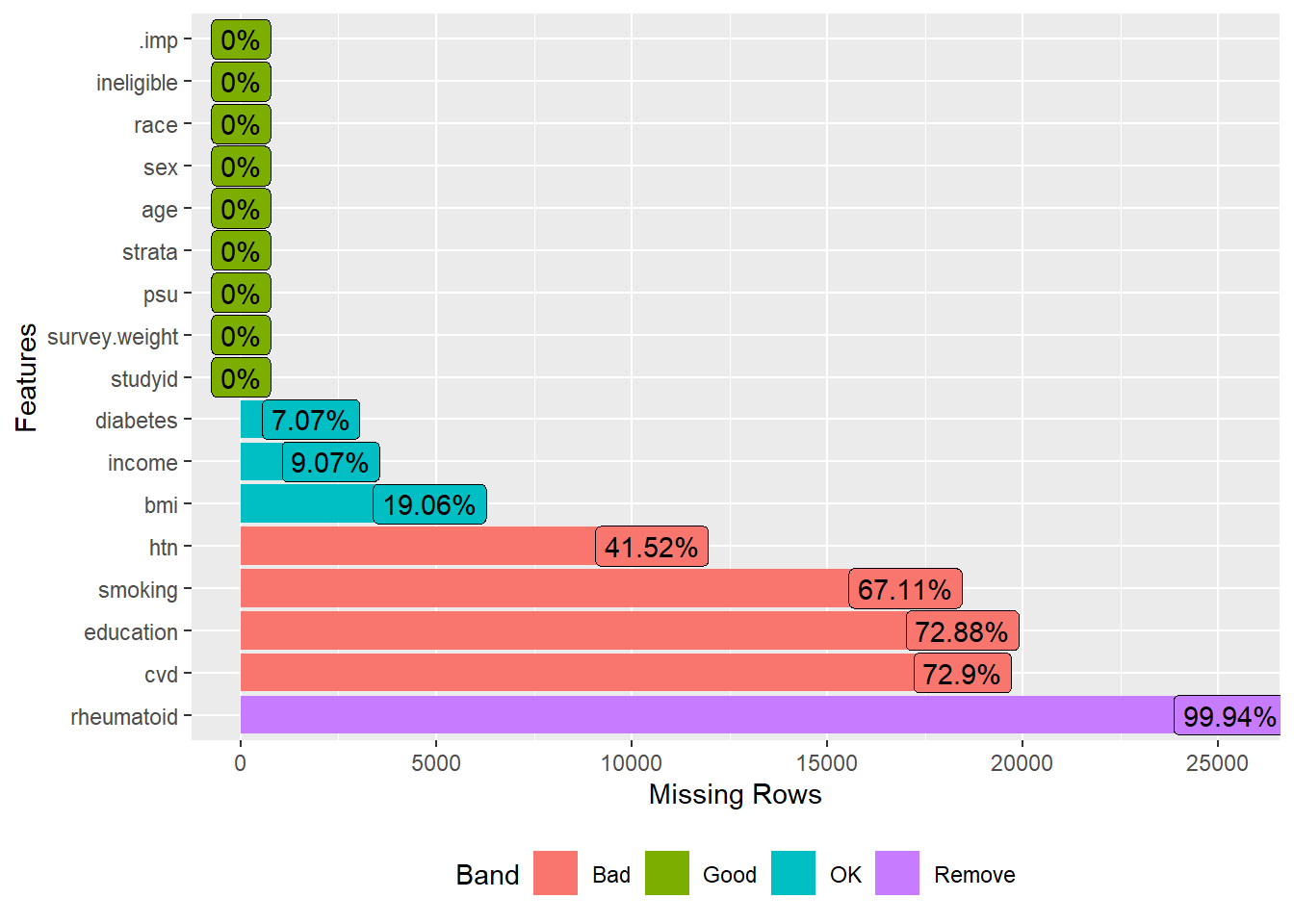
# Stacked data for ineligible subjects
dat.ineligible.stacked <- rbind(dat31, dat32, dat33, dat34, dat35)

We should have missing value in this ineligible part of the data:

DataExplorer::plot_missing(dat.ineligible.stacked)

1.3 Combining eligible (imputed) and ineligible (unimputed) subjects

names(impdata)
#>  [1] ".imp"          "studyid"       "survey.weight" "psu"          
#>  [5] "strata"        "cvd"           "arthritis"     "age.cat"      
#>  [9] "sex"           "education"     "race"          "income"       
#> [13] "bmi"           "smoking"       "htn"           "diabetes"     
#> [17] "ineligible"

names(dat.ineligible.stacked)
#>  [1] "studyid"       "survey.weight" "psu"           "strata"       
#>  [5] "cvd"           "rheumatoid"    "age"           "sex"          
#>  [9] "education"     "race"          "income"        "bmi"          
#> [13] "smoking"       "htn"           "diabetes"      "ineligible"   
#> [17] ".imp"

As we can see, the variable names are different in the two datasets. Particularly, arthritis and age.cat variables are not available in the dat.ineligible.stacked dataset. Now we will recode these variables in the same format as done for impdata:

# Categorical age
summary(dat.ineligible.stacked$age)
#>    Min. 1st Qu.  Median    Mean 3rd Qu.    Max. 
#>    0.00    5.00   12.00   23.25   41.00   80.00
dat.ineligible.stacked$age.cat <- 
  with(dat.ineligible.stacked, 
       ifelse(age >= 20 & age < 50, "20-49", 
              ifelse(age >= 50 & age < 65, "50-64", 
                     ifelse(age >= 65, "65+", NA))))
dat.ineligible.stacked$age.cat <- 
  factor(dat.ineligible.stacked$age.cat, 
         levels = c("20-49", "50-64", "65+"))

Note that, we are assigning anyone with less than 20 age as missing.

table(dat.ineligible.stacked$age.cat, useNA = "always")
#> 
#> 20-49 50-64   65+  <NA> 
#>  1100  2360  3430 18425
# Recode arthritis
dat.ineligible.stacked$arthritis <- 
  car::recode(dat.ineligible.stacked$rheumatoid, 
  " 'No' = 'No arthritis'; 'Yes' = 'Rheumatoid arthritis' ", 
  as.factor = T)

Note: In the above step, we could also create two variables with missing values rather than recoding. The reason is that we will subset the design; no matter whether we recode or create missing values for ineligible, the only information we need from ineligible subjects is their survey features when creating the design.

The next step is to combine these two datasets (impdata and dat.ineligible.stacked).

# Variable names in the imputed dataset
vars <- names(impdata) 

# Set up the dataset for ineligible - same variables as impdata
dat.ineligible.stacked <- dat.ineligible.stacked[, vars]

Now we will merge ineligible and eligible subjects to make the full dataset of 5 $\times$ 9,254 = 46,270 subjects.

impdata2 <- rbind(impdata, dat.ineligible.stacked)
impdata2 <- impdata2[order(impdata2$.imp, impdata2$studyid),]
dim(impdata2)
#> [1] 46270    17

1.4 Prepating Survey design and subpopulation of eligible

The next step is to create the design on full dataset [with eligible (imputed) and ineligible (unimputed) subjects] of 5 $\times$ 9,254 = 46,270 subjects and subset the design for 5 $\times$ 4,716 = 23,580 subjects.

m <- 5
allImputations <- imputationList(lapply(1:m, function(n) 
  subset(impdata2, subset=.imp==n)))

# Step 2: Survey data analysis
w.design0 <- svydesign(ids = ~psu, 
                       weights = ~survey.weight, 
                       strata = ~strata,
                      data = allImputations, 
                      nest = TRUE) # Design on full data
w.design <- subset(w.design0, ineligible == 0) # Subset the design

We can see the length of the subsetted design:

dim(w.design)
#> [1] 4191   17    5

The subsetted design contains 4,191 subjects with 17 variables and 5 imputed datasets. Now we will run the design-adjusted logistic regression on and pool the estimate using Rubin’s rule:

Step 2: Design adjusted regression analysis

# Design-adjusted logistic regression
fit <- with(w.design, 
            svyglm(I(cvd == "Yes") ~ arthritis + age.cat + 
                     sex + education + race + income + bmi + 
                     smoking + htn + diabetes, 
                   family = quasibinomial))
res <- exp(as.data.frame(cbind(coef(fit[[1]]),
      coef(fit[[2]]),
      coef(fit[[3]]),
      coef(fit[[4]]),
      coef(fit[[5]]))))
names(res) <- paste("OR from m =", 1:5)
res.rounded <- round(t(res),2)
kable(res.rounded)

	(Intercept)	arthritisRheumatoid arthritis	age.cat50-64	age.cat65+	sexFemale	educationHigh school	educationCollege graduate or above	raceBlack	raceHispanic	raceOthers	income$20,000 to $74,999	income$75,000 and Over	bmi	smokingPrevious smoker	smokingCurrent smoker	htnYes	diabetesYes
OR from m = 1	0.02	2.03	4.71	13.08	0.46	0.75	0.75	0.96	0.54	0.86	0.48	0.33	1.02	1.55	1.43	1.35	3.01
OR from m = 2	0.02	2.04	4.74	13.21	0.45	0.76	0.79	0.97	0.54	0.88	0.48	0.32	1.03	1.55	1.47	1.30	3.01
OR from m = 3	0.02	2.12	4.58	11.88	0.47	0.71	0.70	0.98	0.54	0.85	0.54	0.36	1.01	1.59	1.45	1.48	3.13
OR from m = 4	0.02	2.10	4.59	12.45	0.46	0.70	0.71	0.96	0.53	0.86	0.51	0.34	1.02	1.56	1.44	1.46	3.03
OR from m = 5	0.02	2.07	4.47	12.25	0.45	0.75	0.77	0.99	0.55	0.87	0.53	0.34	1.02	1.55	1.45	1.47	3.05

Step 3: Pooling estimates

# Step 3: Pooled estimates
pooled.estimates <- MIcombine(fit)
OR <- round(exp(pooled.estimates$coefficients), 2)
OR <- as.data.frame(OR)
CI <- round(exp(confint(pooled.estimates)), 2)
OR <- cbind(OR, CI)
OR

Conclusion

Among US adults aged 20 years or more, the odds of CVD was approximately twice among those with rheumatoid arthritis than no arthritis.

References

Hossain, Md Belal, Jacek A Kopec, Mohammad Atiquzzaman, and Mohammad Ehsanul Karim. 2022. “The Association Between Rheumatoid Arthritis and Cardiovascular Disease Among Adults in the United States During 1999–2018, and Age-Related Effect Modification in Relative and Absolute Scales.” Annals of Epidemiology 71: 23–30.