PSM with MI

The tutorial provides a detailed walkthrough of implementing Propensity Score Matching (PSM) combined with Multiple Imputation (MI) in a statistical analysis, focusing on handling missing data and mitigating bias in observational studies.

The initial chunk is dedicated to loading various R packages that will be utilized throughout the tutorial. These libraries provide functions and tools that facilitate data manipulation, statistical modeling, visualization, and more.

# Load required packages
library(MatchIt)
require(tableone)
require(survey)
require(cobalt)
require(Publish)
require(optmatch)
require(data.table)
require(jtools)
require(ggstance)
require(DataExplorer)
require(mitools)
library(kableExtra)
library(mice)

Problem Statement

Logistic regression

Perform multiple imputation to deal with missing values; with 3 imputed datasets, 5 iterations,
fit survey featured logistic regression in all of the 3 imputed datasets, and
obtain the pooled OR (adjusted) and the corresponding 95% confidence intervals.
Hints
- Use the covariates (listed below) in the imputation model.
- Imputation model covariates can be different than the original analysis covariates. You are encouraged to use variables in the imputation model that can be predictive of the variables with missing observations. In this example, we use the strata variable as an auxiliary variable in the imputation model, but not the survey weight or PSU variable.
- Also the imputation model specification can be modified. For example, we use pmm method for bmi in the imputation model.
- Remove any subject ID variable from the imputation model, if created in an intermediate step. Indeed ID variables should not be in the imputation model, if they are not predictive of the variables with missing observations.

Tip

Predictive Mean Matching:

The “Predictive Mean Matching” (PMM) method in Multiple Imputation (MI) is a widely used technique to handle missing data, particularly well-suited for continuous variables. PMM operates by first creating a predictive model for the variable with missing data, using observed values from other variables in the dataset. For each missing value, PMM identifies a set of observed values with predicted scores that are close to the predicted score for the missing value, derived from the predictive model. Then, instead of imputing a predicted score directly, PMM randomly selects one of the observed values from this set and assigns it as the imputed value. This method retains the original distribution of the imputed variable since it only uses observed values for imputation, and it also tends to preserve relationships between variables. PMM is particularly advantageous when the normality assumption of the imputed variable is questionable, providing a robust and practical approach to managing missing data in various research contexts.

Propensity score matching (Zanutto, 2006)

Use the propensity score matching as per Zanutto E. L. (2006)’s recommendation in all of the imputed datasets.
Report the pooled OR estimates (adjusted) and corresponding 95% confidence intervals (adjusted OR).

Data and variables

Analytic data

The analytic dataset is saved as NHANES17.RData.

Variables

We are primarily interested in outcome diabetes and exposure whether born in the US (born).

Variables under consideration:

survey features
- PSU
- strata
- survey weight
Covariates
- race
- age
- marriage
- education
- gender
- BMI
- systolic blood pressure

Pre-processing

The data is loaded and variables of interest are identified.

load(file="Data/propensityscore/NHANES17.RData") # read data
ls()
#> [1] "analytic"           "analytic.with.miss" "has_annotations"
dim(analytic.with.miss)
#> [1] 9254   34
vars <- c("ID", # ID
          "psu", "strata", "weight", # Survey features 
          "race", "age", "married","education","gender","bmi","systolicBP", # Covariates
          "born", # Exposure
          "diabetes") # Outcome

Subset the dataset

The dataset is then subsetted to retain only the relevant variables, ensuring that subsequent analyses are focused and computationally efficient.

dat.with.miss <- analytic.with.miss[,vars]
dim(analytic.with.miss)
#> [1] 9254   34

Inspect weights

The weights of the observations are inspected and adjusted to avoid issues in subsequent analyses.

summary(dat.with.miss$weight)
#>    Min. 1st Qu.  Median    Mean 3rd Qu.    Max. 
#>       0   12347   21060   34671   37562  419763
# weight = 0 would create problem in the analysis
# ad-hoc solution to 0 weight problem
dat.with.miss$weight[dat.with.miss$weight == 0] <- 0.00000001

Recode the exposure variable

The exposure variable is recoded for clarity and ease of interpretation in results.

dat.with.miss$born <- car::recode(dat.with.miss$born, 
recodes = " 'Born in 50 US states or Washingt' = 
'Born in US'; 'Others' = 'Others'; else = NA " )
dat.with.miss$born <- factor(dat.with.miss$born, levels = c("Born in US", "Others"))

variable types

Variable types are set, ensuring that each variable is treated appropriately in the analyses.

factor.names <- c("race", "married", "education", "gender", "diabetes")
dat.with.miss[,factor.names] <- lapply(dat.with.miss[,factor.names], factor)

Inspect extent of missing data problem

A visualization is generated to explore the extent and pattern of missing data in the dataset, which informs the strategy for handling them.

require(DataExplorer)
plot_missing(dat.with.miss)

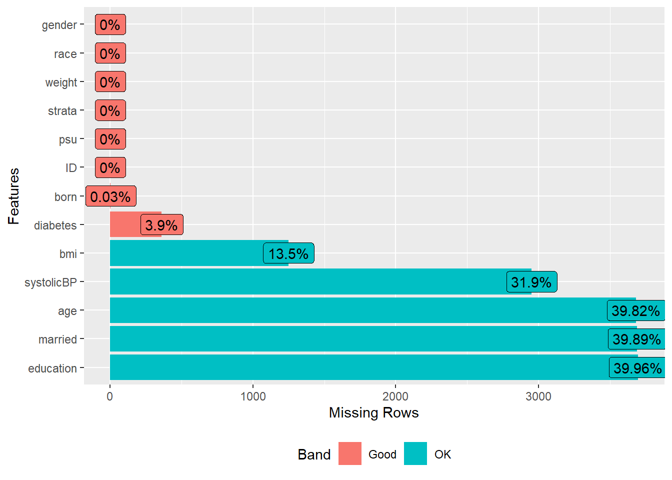
Note that, multiple imputation then delete (MID) approach can be applied if the outcome had some missing values. Due to the small number of missingness, MICE may not impute the outcomes BTW.

Tip

Multiple imputation then delete (MID):

MID is a specific approach used in the context of multiple imputation (MI) when dealing with missing outcome data. All missing values, including those in the outcome variable, are imputed to create several complete datasets. In subsequent analyses, the imputed values for the outcome variable are deleted, so that only observed outcome values are analyzed. Each dataset (with observed outcome values and imputed predictor values) is analyzed separately, and results are pooled to provide a single estimate.

Logistic regression

Initialization

The MI process is initialized, setting up the framework for subsequent imputations.

imputation <- mice(data = dat.with.miss, maxit = 0, print = FALSE)

Setting imputation model covariates

The predictor matrix is adjusted to specify which variables will be used to predict missing values in the imputation model. Setting strata as auxiliary variable:

pred <- imputation$pred
pred
#>            ID psu strata weight race age married education gender bmi
#> ID          0   1      1      1    1   1       1         1      1   1
#> psu         1   0      1      1    1   1       1         1      1   1
#> strata      1   1      0      1    1   1       1         1      1   1
#> weight      1   1      1      0    1   1       1         1      1   1
#> race        1   1      1      1    0   1       1         1      1   1
#> age         1   1      1      1    1   0       1         1      1   1
#> married     1   1      1      1    1   1       0         1      1   1
#> education   1   1      1      1    1   1       1         0      1   1
#> gender      1   1      1      1    1   1       1         1      0   1
#> bmi         1   1      1      1    1   1       1         1      1   0
#> systolicBP  1   1      1      1    1   1       1         1      1   1
#> born        1   1      1      1    1   1       1         1      1   1
#> diabetes    1   1      1      1    1   1       1         1      1   1
#>            systolicBP born diabetes
#> ID                  1    1        1
#> psu                 1    1        1
#> strata              1    1        1
#> weight              1    1        1
#> race                1    1        1
#> age                 1    1        1
#> married             1    1        1
#> education           1    1        1
#> gender              1    1        1
#> bmi                 1    1        1
#> systolicBP          0    1        1
#> born                1    0        1
#> diabetes            1    1        0
pred[,"ID"] <- pred["ID",] <- 0
pred[,"psu"] <- pred["psu",] <- 0
pred[,"weight"] <- pred["weight",] <- 0
pred["strata",] <- 0
pred
#>            ID psu strata weight race age married education gender bmi
#> ID          0   0      0      0    0   0       0         0      0   0
#> psu         0   0      0      0    0   0       0         0      0   0
#> strata      0   0      0      0    0   0       0         0      0   0
#> weight      0   0      0      0    0   0       0         0      0   0
#> race        0   0      1      0    0   1       1         1      1   1
#> age         0   0      1      0    1   0       1         1      1   1
#> married     0   0      1      0    1   1       0         1      1   1
#> education   0   0      1      0    1   1       1         0      1   1
#> gender      0   0      1      0    1   1       1         1      0   1
#> bmi         0   0      1      0    1   1       1         1      1   0
#> systolicBP  0   0      1      0    1   1       1         1      1   1
#> born        0   0      1      0    1   1       1         1      1   1
#> diabetes    0   0      1      0    1   1       1         1      1   1
#>            systolicBP born diabetes
#> ID                  0    0        0
#> psu                 0    0        0
#> strata              0    0        0
#> weight              0    0        0
#> race                1    1        1
#> age                 1    1        1
#> married             1    1        1
#> education           1    1        1
#> gender              1    1        1
#> bmi                 1    1        1
#> systolicBP          0    1        1
#> born                1    0        1
#> diabetes            1    1        0

Setting imputation model specification

The method for imputing a particular variable is specified (e.g., using Predictive Mean Matching). Here, we add pmm for bmi:

meth <- imputation$meth
meth["bmi"] <- "pmm"

Impute incomplete data

Multiple datasets are imputed, each providing a different “guess” at the missing values, based on observed data. We are imputing m = 3 times.

imputation <- mice(data = dat.with.miss, 
                   seed = 123, 
                   predictorMatrix = pred,
                   method = meth, 
                   m = 3, 
                   maxit = 5, 
                   print = FALSE)
impdata <- mice::complete(imputation, action="long")
impdata$.id <- NULL
m <- 3
set.seed(123)
allImputations <-  imputationList(lapply(1:m, 
                                         function(n)
                                           subset(impdata, 
                                                  subset=.imp==n)))
str(allImputations)
#> List of 2
#>  $ imputations:List of 3
#>   ..$ :'data.frame': 9254 obs. of  14 variables:
#>   .. ..$ .imp      : int [1:9254] 1 1 1 1 1 1 1 1 1 1 ...
#>   .. ..$ ID        : int [1:9254] 93703 93704 93705 93706 93707 93708 93709 93710 93711 93712 ...
#>   .. ..$ psu       : Factor w/ 2 levels "1","2": 2 1 2 2 1 2 1 1 2 2 ...
#>   .. ..$ strata    : Factor w/ 15 levels "134","135","136",..: 12 10 12 1 5 5 3 1 1 14 ...
#>   .. ..$ weight    : num [1:9254] 8540 42567 8338 8723 7065 ...
#>   .. ..$ race      : Factor w/ 4 levels "Black","Hispanic",..: 3 4 1 3 3 3 1 4 3 2 ...
#>   .. ..$ age       : int [1:9254] 57 46 66 50 23 66 75 49 56 36 ...
#>   .. ..$ married   : Factor w/ 3 levels "Married","Never.married",..: 1 1 3 1 2 1 3 3 1 1 ...
#>   .. ..$ education : Factor w/ 3 levels "College","High.School",..: 1 2 2 1 1 3 1 2 1 3 ...
#>   .. ..$ gender    : Factor w/ 2 levels "Female","Male": 1 2 1 2 2 1 1 1 2 2 ...
#>   .. ..$ bmi       : num [1:9254] 17.5 15.7 31.7 21.5 18.1 23.7 38.9 31.2 21.3 19.7 ...
#>   .. ..$ systolicBP: int [1:9254] 108 96 200 112 128 124 120 122 108 112 ...
#>   .. ..$ born      : Factor w/ 2 levels "Born in US","Others": 1 1 1 1 1 2 1 1 2 2 ...
#>   .. ..$ diabetes  : Factor w/ 2 levels "No","Yes": 1 1 1 1 1 2 1 1 1 1 ...
#>   ..$ :'data.frame': 9254 obs. of  14 variables:
#>   .. ..$ .imp      : int [1:9254] 2 2 2 2 2 2 2 2 2 2 ...
#>   .. ..$ ID        : int [1:9254] 93703 93704 93705 93706 93707 93708 93709 93710 93711 93712 ...
#>   .. ..$ psu       : Factor w/ 2 levels "1","2": 2 1 2 2 1 2 1 1 2 2 ...
#>   .. ..$ strata    : Factor w/ 15 levels "134","135","136",..: 12 10 12 1 5 5 3 1 1 14 ...
#>   .. ..$ weight    : num [1:9254] 8540 42567 8338 8723 7065 ...
#>   .. ..$ race      : Factor w/ 4 levels "Black","Hispanic",..: 3 4 1 3 3 3 1 4 3 2 ...
#>   .. ..$ age       : int [1:9254] 24 49 66 32 34 66 75 80 56 28 ...
#>   .. ..$ married   : Factor w/ 3 levels "Married","Never.married",..: 2 1 3 2 1 1 3 3 1 2 ...
#>   .. ..$ education : Factor w/ 3 levels "College","High.School",..: 1 1 2 1 2 3 1 1 1 1 ...
#>   .. ..$ gender    : Factor w/ 2 levels "Female","Male": 1 2 1 2 2 1 1 1 2 2 ...
#>   .. ..$ bmi       : num [1:9254] 17.5 15.7 31.7 21.5 18.1 23.7 38.9 24.9 21.3 19.7 ...
#>   .. ..$ systolicBP: int [1:9254] 102 104 136 112 128 120 120 120 108 112 ...
#>   .. ..$ born      : Factor w/ 2 levels "Born in US","Others": 1 1 1 1 1 2 1 1 2 2 ...
#>   .. ..$ diabetes  : Factor w/ 2 levels "No","Yes": 1 1 1 1 1 2 1 1 1 1 ...
#>   ..$ :'data.frame': 9254 obs. of  14 variables:
#>   .. ..$ .imp      : int [1:9254] 3 3 3 3 3 3 3 3 3 3 ...
#>   .. ..$ ID        : int [1:9254] 93703 93704 93705 93706 93707 93708 93709 93710 93711 93712 ...
#>   .. ..$ psu       : Factor w/ 2 levels "1","2": 2 1 2 2 1 2 1 1 2 2 ...
#>   .. ..$ strata    : Factor w/ 15 levels "134","135","136",..: 12 10 12 1 5 5 3 1 1 14 ...
#>   .. ..$ weight    : num [1:9254] 8540 42567 8338 8723 7065 ...
#>   .. ..$ race      : Factor w/ 4 levels "Black","Hispanic",..: 3 4 1 3 3 3 1 4 3 2 ...
#>   .. ..$ age       : int [1:9254] 47 71 66 71 45 66 75 37 56 47 ...
#>   .. ..$ married   : Factor w/ 3 levels "Married","Never.married",..: 1 1 3 1 1 1 3 1 1 1 ...
#>   .. ..$ education : Factor w/ 3 levels "College","High.School",..: 1 1 2 1 1 3 1 1 1 2 ...
#>   .. ..$ gender    : Factor w/ 2 levels "Female","Male": 1 2 1 2 2 1 1 1 2 2 ...
#>   .. ..$ bmi       : num [1:9254] 17.5 15.7 31.7 21.5 18.1 23.7 38.9 15.9 21.3 19.7 ...
#>   .. ..$ systolicBP: int [1:9254] 100 114 162 112 128 166 120 116 108 112 ...
#>   .. ..$ born      : Factor w/ 2 levels "Born in US","Others": 1 1 1 1 1 2 1 1 2 2 ...
#>   .. ..$ diabetes  : Factor w/ 2 levels "No","Yes": 1 1 1 1 1 2 1 1 1 1 ...
#>  $ call       : language imputationList(lapply(1:m, function(n) subset(impdata, subset = .imp ==      n)))
#>  - attr(*, "class")= chr "imputationList"

Design

A survey design object is created, ensuring that subsequent analyses appropriately account for the survey design.

w.design <- svydesign(ids = ~psu, weights = ~weight, strata = ~strata,
                      data = allImputations, nest = TRUE)

Survey data analysis

A logistic regression model is fitted to each imputed dataset.

model.formula <- as.formula(I(diabetes == 'Yes') ~ 
                              born + race + age + married + 
                              education + gender + bmi + systolicBP)
fit.from.logistic <- with(w.design, svyglm(model.formula, family = binomial("logit")))
#> Warning in eval(family$initialize): non-integer #successes in a binomial glm!

#> Warning in eval(family$initialize): non-integer #successes in a binomial glm!

#> Warning in eval(family$initialize): non-integer #successes in a binomial glm!

Pooled estimates

Results from models across all imputed datasets are pooled to provide a single estimate, accounting for the uncertainty due to missing data.

pooled.estimates <- MIcombine(fit.from.logistic)
summary(pooled.estimates, digits = 2, logeffect=TRUE)
#> Multiple imputation results:
#>       with(w.design, svyglm(model.formula, family = binomial("logit")))
#>       MIcombine.default(fit.from.logistic)
#>                           results      se  (lower  upper) missInfo
#> (Intercept)               0.00013 7.5e-05 3.9e-05 0.00041     22 %
#> bornOthers                1.44729 2.7e-01 1.0e+00 2.07384      0 %
#> raceHispanic              0.81619 1.1e-01 6.3e-01 1.05882      0 %
#> raceOther                 1.43817 2.6e-01 1.0e+00 2.04954      3 %
#> raceWhite                 0.86411 1.3e-01 6.5e-01 1.14994      3 %
#> age                       1.06157 3.6e-03 1.1e+00 1.06874      6 %
#> marriedNever.married      0.83242 1.6e-01 5.7e-01 1.20809     10 %
#> marriedPreviously.married 0.88401 1.1e-01 6.8e-01 1.14163     11 %
#> educationHigh.School      1.16331 1.9e-01 8.4e-01 1.60803      0 %
#> educationSchool           1.41943 2.4e-01 1.0e+00 1.98397      7 %
#> genderMale                1.53458 1.8e-01 1.2e+00 1.94217      3 %
#> bmi                       1.10597 1.2e-02 1.1e+00 1.12956      1 %
#> systolicBP                1.00325 3.2e-03 1.0e+00 1.01001     39 %
OR <- round(exp(pooled.estimates$coefficients), 2) 
OR <- as.data.frame(OR)
CI <- round(exp(confint(pooled.estimates)), 2)
OR <- cbind(OR, CI)
OR[2,]

Propensity score matching analysis

Initialization

The MI process is re-initialized to facilitate PSM in the context of MI.

imputation <- mice(data = dat.with.miss, maxit = 0, print = FALSE)
impdata <- mice::complete(imputation, action="long")
m <- 3
allImputations <- imputationList(lapply(1:m, 
                                        function(n) 
                                          subset(impdata, 
                                                 subset=.imp==n)))

Zanutto E. L. (2006) under multiple imputation

Tip

An iterative process is performed within each imputed dataset, which involves:

Estimating propensity scores.
Matching treated and untreated subjects based on these scores.
Extracting matched data and checking the balance of covariates across matched groups.
Fitting outcome models to the survey weighted matched data and estimating treatment effects.

Notice that we are performing multi-step process within MI

match.statm <- SMDm <- tab1m <- vector("list", m) 
fit.from.PS <- vector("list", m)

for (i in 1:m) {
  analytic.i <- allImputations$imputations[[i]]
  # Rename the weight variable into survey.weight
  names(analytic.i)[names(analytic.i) == "weight"] <- "survey.weight"
  
  # Specify the PS model to estimate propensity scores
  ps.formula <- as.formula(I(born=="Others") ~ 
                             race + age + married + education + 
                             gender + bmi + systolicBP)

  # Propensity scores
  ps.fit <- glm(ps.formula, data = analytic.i, family = binomial("logit"))
  analytic.i$PS <- fitted(ps.fit)
  
  # Match exposed and unexposed subjects 
  set.seed(123)
  match.obj <- matchit(ps.formula, data = analytic.i, 
                       distance = analytic.i$PS, 
                       method = "nearest", 
                       replace = FALSE,
                       caliper = 0.2, 
                       ratio = 1)
  match.statm[[i]] <- match.obj
  analytic.i$PS <- match.obj$distance
  
  # Extract matched data
  matched.data <- match.data(match.obj) 
  
  # Balance checking
  cov <- c("race", "age", "married", "education", "gender", "bmi", "systolicBP")
  
  tab1m[[i]] <- CreateTableOne(strata = "born", 
                               vars = cov, data = matched.data, 
                               test = FALSE, smd = TRUE)
  SMDm[[i]] <- ExtractSmd(tab1m[[i]])
  
  # Setup the design with survey features
  analytic.i$matched <- 0
  analytic.i$matched[analytic.i$ID %in% matched.data$ID] <- 1
  
  # Survey setup for full data
  w.design0 <- svydesign(strata = ~strata, id = ~psu, weights = ~survey.weight, 
                         data = analytic.i, nest = TRUE)
  
  # Subset matched data
  w.design.m <- subset(w.design0, matched == 1)
  
  # Outcome model (double adjustment)
  out.formula <- as.formula(I(diabetes == "Yes") ~ 
                              born + race + age + married + 
                              education + gender + bmi + systolicBP)
  fit.from.PS[[i]] <- svyglm(out.formula, design = w.design.m, 
                     family = quasibinomial("logit"))
}

Check matched data

The matched data is inspected to ensure that matching was successful and appropriate.

match.statm
#> [[1]]
#> A matchit object
#>  - method: 1:1 nearest neighbor matching without replacement
#>  - distance: User-defined [caliper]
#>  - caliper: <distance> (0.044)
#>  - number of obs.: 9254 (original), 3590 (matched)
#>  - target estimand: ATT
#>  - covariates: race, age, married, education, gender, bmi, systolicBP
#> 
#> [[2]]
#> A matchit object
#>  - method: 1:1 nearest neighbor matching without replacement
#>  - distance: User-defined [caliper]
#>  - caliper: <distance> (0.044)
#>  - number of obs.: 9254 (original), 3598 (matched)
#>  - target estimand: ATT
#>  - covariates: race, age, married, education, gender, bmi, systolicBP
#> 
#> [[3]]
#> A matchit object
#>  - method: 1:1 nearest neighbor matching without replacement
#>  - distance: User-defined [caliper]
#>  - caliper: <distance> (0.044)
#>  - number of obs.: 9254 (original), 3594 (matched)
#>  - target estimand: ATT
#>  - covariates: race, age, married, education, gender, bmi, systolicBP

Check balance in matched data

The balance of covariates across matched groups is assessed to ensure that matching has successfully reduced bias.

SMDm
#> [[1]]
#>                 1 vs 2
#> race       0.028883793
#> age        0.033614763
#> married    0.007318561
#> education  0.117536503
#> gender     0.040145831
#> bmi        0.043350560
#> systolicBP 0.054549772
#> 
#> [[2]]
#>                 1 vs 2
#> race       0.019901420
#> age        0.016267050
#> married    0.017196043
#> education  0.128811588
#> gender     0.003338016
#> bmi        0.057014434
#> systolicBP 0.071553721
#> 
#> [[3]]
#>                1 vs 2
#> race       0.04490482
#> age        0.01959377
#> married    0.03687394
#> education  0.13301810
#> gender     0.01225625
#> bmi        0.03697878
#> systolicBP 0.10025529

Pooled estimate

Finally, the treatment effect estimates from the matched analyses across all imputed datasets are pooled to provide a single, overall estimate, ensuring that the final result appropriately accounts for the uncertainty due to both the matching process and the imputation of missing data.

pooled.estimates <- MIcombine(fit.from.PS)
summary(pooled.estimates, digits = 2, logeffect=TRUE)
#> Multiple imputation results:
#>       MIcombine.default(fit.from.PS)
#>                           results      se  (lower  upper) missInfo
#> (Intercept)               8.9e-05 4.9e-05 0.00003 0.00026      8 %
#> bornOthers                2.0e+00 3.1e-01 1.47719 2.73325     16 %
#> raceHispanic              7.0e-01 1.7e-01 0.42593 1.15504     27 %
#> raceOther                 1.4e+00 4.1e-01 0.77209 2.53278     26 %
#> raceWhite                 4.9e-01 2.7e-01 0.15853 1.52308     28 %
#> age                       1.1e+00 4.6e-03 1.04472 1.06298      8 %
#> marriedNever.married      5.9e-01 2.0e-01 0.28824 1.18926     38 %
#> marriedPreviously.married 1.0e+00 2.5e-01 0.62417 1.64438     11 %
#> educationHigh.School      1.4e+00 3.0e-01 0.89403 2.10852      2 %
#> educationSchool           1.3e+00 3.4e-01 0.81042 2.21438      7 %
#> genderMale                1.3e+00 2.3e-01 0.86695 1.83880     31 %
#> bmi                       1.1e+00 1.1e-02 1.08062 1.12285      5 %
#> systolicBP                1.0e+00 3.0e-03 1.00314 1.01494      3 %
OR <- round(exp(pooled.estimates$coefficients), 2) 
OR <- as.data.frame(OR)
CI <- round(exp(confint(pooled.estimates)), 2)
OR <- cbind(OR, CI)
OR[2,]