Collapsibility

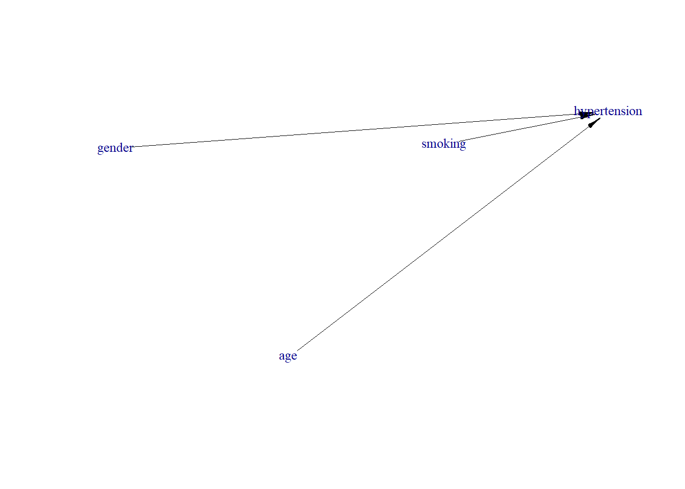
Let us assume we have a regression of hypertension (\(Y\)), smoking (\(A\)) and a risk factor for outcome, gender (\(L\)). Then let us set up 2 regression models:

• 1st regression model is \(Y \sim \beta \times A + \alpha \times L\). Here we are conditioning on gender (\(L\)).
• 2nd regression model is \(Y \sim \beta' \times A\)

Then regression is collapsible for \(\beta\) over \(L\) if \(\beta = \beta'\) from the 2nd regression omitting \(L\). \(\beta \ne \beta'\) would mean non-collapsibility. A measure of association (say, risk difference) is collapsible if the marginal measure of association is equal to a weighted average of the stratum-specific measures of association. Non-collapsibility is also knows as Simpson’s Paradox (in absence of confounding of course): a statistical phenomenon where an association between two factors (say, hypertension and smoking) in a population (we are talking about marginal estimate here) is different than the associations of same relationship in subpopulations (conditional on some other factor, say, age; hence talking about conditional estimates). Risk ratio and risk difference are collapsible.

Odds ratio can be non-collapsible. It can produce different treatment effect estimate for different covariate adjustment sets (see example below of when adjusting form age and sex vs. when adjusting none). This is true even in the absence of confounding. However, according to our definition here, OR is collapsible when we consider gender in the adjustment set.

Note that, OR non-collapsibility is a consequence of the fact that it is estimated via a logit link function (nonlinearity of the logistic transformation).

Ref:

• (Greenland, Pearl, and Robins 1999)
• (Mansournia and Greenland 2015)

# Load required packages
library(simcausal)
library(tableone)
library(Publish)
library(lawstat)

Data generating process

Let us generate the data with smoking being the exposure and hypertension being the outcome.

require(simcausal)
D <- DAG.empty()
D <- D + 
  node("gender", distr = "rbern", prob = 0.7) +
  node("age", distr = "rnorm", mean = 2, sd = 4) +
  node("smoking", distr = "rbern", prob = plogis(.1)) +
  node("hypertension", distr = "rbern", 
       prob = plogis(1 + log(3.5) * smoking + log(.1) * gender + log(7) * age))
Dset <- set.DAG(D)

Generate DAG

plotDAG(Dset, xjitter = 0.1, yjitter = .9,
        edge_attrs = list(width = 0.5, arrow.width = 0.4, arrow.size = 0.7),
        vertex_attrs = list(size = 12, label.cex = 0.8))

Generate Data

Obs.Data <- sim(DAG = Dset, n = 100000, rndseed = 123)
head(Obs.Data)

Balance check

require(tableone)
CreateTableOne(data = Obs.Data, strata = "smoking", vars = c("gender", "age"))
#>                     Stratified by smoking
#>                      0            1            p      test
#>   n                  47720        52280                   
#>   gender (mean (SD))  0.70 (0.46)  0.70 (0.46)  0.403     
#>   age (mean (SD))     2.02 (4.02)  2.01 (4.00)  0.690

Conditional and crude risk difference (RD)

Since RD is a collapsible measure, the marginal and conditional estimate should be approximately the same.

Full list of risk factors for outcome (2 variables)

## RD
require(Publish)
fitx0 <- glm(hypertension ~ smoking + gender + age, 
             family=gaussian(link = "identity"), data=Obs.Data)
publish(fitx0, print = FALSE, confint.method = "robust", 
        pvalue.method = "robust")$regressionTable[2,]

Ref:

• (Naimi and Whitcomb 2020) (“For the risk difference, one may use a GLM with a Gaussian (i.e., normal) distribution and identity link function, or, equivalently, an ordinary least squares estimator …robust variance estimator (or bootstrap) should be used to obtain valid standard errors.”)

Strtatum specific (2 variables)

fitx1 <- glm(hypertension ~ smoking, family=gaussian(link = "identity"), 
             data=subset(Obs.Data, gender == 1 & age < 2))
publish(fitx1, print = FALSE, confint.method = "robust", 
        pvalue.method = "robust")$regressionTable[2,]

fitx2 <- glm(hypertension ~ smoking, family=gaussian(link = "identity"), 
             data=subset(Obs.Data, gender == 0 & age < 2))
publish(fitx2, print = FALSE, confint.method = "robust", 
        pvalue.method = "robust")$regressionTable[2,]

fitx3 <- glm(hypertension ~ smoking, family=gaussian(link = "identity"), 
             data=subset(Obs.Data, gender == 1 & age >= 2))
publish(fitx3, print = FALSE, confint.method = "robust", 
        pvalue.method = "robust")$regressionTable[2,]

fitx4 <- glm(hypertension ~ smoking, family=gaussian(link = "identity"), 
             data=subset(Obs.Data, gender == 0 & age >= 2))
publish(fitx4, print = FALSE, confint.method = "robust", 
        pvalue.method = "robust")$regressionTable[2,]

Unweighted mean from all strata (for simplicity, 2 variables)

round(mean(c(coef(fitx1)["smoking"],
             coef(fitx2)["smoking"],
             coef(fitx3)["smoking"],
             coef(fitx4)["smoking"])),2)
#> [1] 0.05

Partial list of risk factors for outcome (1 variable)

fitx0 <- glm(hypertension ~ smoking + gender, 
             family=gaussian(link = "identity"), data=Obs.Data)
publish(fitx0, print = FALSE, confint.method = "robust", 
        pvalue.method = "robust")$regressionTable[2,]

Strtatum specific (1 variable)

fitx1 <- glm(hypertension ~ smoking, family=gaussian(link = "identity"), 
             data=subset(Obs.Data, gender == 1))
publish(fitx1, print = FALSE, confint.method = "robust", 
        pvalue.method = "robust")$regressionTable[2,]

fitx2 <- glm(hypertension ~ smoking, family=gaussian(link = "identity"), 
             data=subset(Obs.Data, gender == 0))
publish(fitx2, print = FALSE, confint.method = "robust", 
        pvalue.method = "robust")$regressionTable[2,]

Unweighted mean from all strata (for simplicity, 1 variable)

round(mean(c(coef(fitx1)["smoking"],
             coef(fitx2)["smoking"])),2)
#> [1] 0.05

Crude (in absence of confounding)

fitx0 <- glm(hypertension ~ smoking, 
             family=gaussian(link = "identity"), data=Obs.Data)
publish(fitx0, print = FALSE, confint.method = "robust", 
        pvalue.method = "robust")$regressionTable[2,]

Conditional and crude risk ratio (RR)

Ref:

• (Naimi and Whitcomb 2020) (“For the risk ratio, one may use a GLM with a Poisson distribution and log link function …. one should use the robust (or sandwich) variance estimator to obtain valid standard errors (the bootstrap can also be used)”).

Full list of risk factors for outcome (2 variables)

fitx0 <- glm(hypertension ~ smoking + gender + age, 
             family=poisson(link = "log"), data=Obs.Data)
publish(fitx0, print = FALSE, confint.method = "robust", 
        pvalue.method = "robust")$regressionTable[1,]

The estimate we see as a hazard ratio is basically a risk ratio.

Strtatum specific (2 variables)

fitx1 <- glm(hypertension ~ smoking, 
             family=poisson(link = "log"), 
             data=subset(Obs.Data, gender == 1 & age < 2))
publish(fitx1, print = FALSE, confint.method = "robust", 
        pvalue.method = "robust")$regressionTable[1,]

fitx2 <- glm(hypertension ~ smoking, 
             family=poisson(link = "log"), 
             data=subset(Obs.Data, gender == 0 & age < 2))
publish(fitx2, print = FALSE, confint.method = "robust", 
        pvalue.method = "robust")$regressionTable[1,]

fitx3 <- glm(hypertension ~ smoking, 
             family=poisson(link = "log"), 
             data=subset(Obs.Data, gender == 1 & age >= 2))
publish(fitx3, print = FALSE, confint.method = "robust", 
        pvalue.method = "robust")$regressionTable[1,]

fitx4 <- glm(hypertension ~ smoking, 
             family=poisson(link = "log"), 
             data=subset(Obs.Data, gender == 0 & age >= 2))
publish(fitx4, print = FALSE, confint.method = "robust", 
        pvalue.method = "robust")$regressionTable[1,]

Unweighted mean from all strata (for simplicity, 2 variables)

mean(exp(c(coef(fitx1)["smoking"],
           coef(fitx2)["smoking"],
           coef(fitx3)["smoking"],
           coef(fitx4)["smoking"])))
#> [1] 1.156387

Partial list of risk factors for outcome (1 variable)

fitx0 <- glm(hypertension ~ smoking + gender, 
             family=poisson(link = "log"), data=Obs.Data)
publish(fitx0, print = FALSE, confint.method = "robust", 
        pvalue.method = "robust")$regressionTable[1,]

Strtatum specific (1 variable)

fitx1 <- glm(hypertension ~ smoking, 
             family=poisson(link = "log"), 
             data=subset(Obs.Data, gender == 1))
publish(fitx1, print = FALSE, confint.method = "robust", 
        pvalue.method = "robust")$regressionTable[1,]

fitx2 <- glm(hypertension ~ smoking, 
             family=poisson(link = "log"), 
             data=subset(Obs.Data, gender == 0))
publish(fitx2, print = FALSE, confint.method = "robust", 
        pvalue.method = "robust")$regressionTable[1,]

Unweighted mean from all strata (for simplicity, 1 variable)

mean(exp(c(coef(fitx1)["smoking"],
           coef(fitx2)["smoking"])))
#> [1] 1.077402

Crude (in absence of confounding)

fitx0 <- glm(hypertension ~ smoking, 
             family=poisson(link = "log"), data=Obs.Data)
publish(fitx0, print = FALSE, confint.method = "robust", 
        pvalue.method = "robust")$regressionTable[1,]

Since the marginal and conditional estimate are approximately the same, RD is a collapsible measure.

Conditional and crude OR

Full list of risk factors for outcome (2 variables)

fitx0 <- glm(hypertension ~ smoking + gender + age, family=binomial(link = "logit"), data=Obs.Data)
publish(fitx0, print = FALSE, confint.method = "robust", pvalue.method = "robust")$regressionTable[1,]

Strtatum specific (2 variables)

fitx1 <- glm(hypertension ~ smoking, 
             family=binomial(link = "logit"), 
             data=subset(Obs.Data, gender == 1 & age < 2))
publish(fitx1, print = FALSE, confint.method = "robust", 
        pvalue.method = "robust")$regressionTable[1,]

fitx2 <- glm(hypertension ~ smoking, 
             family=binomial(link = "logit"), 
             data=subset(Obs.Data, gender == 0 & age < 2))
publish(fitx2, print = FALSE, confint.method = "robust", 
        pvalue.method = "robust")$regressionTable[1,]

fitx3 <- glm(hypertension ~ smoking, 
             family=binomial(link = "logit"), 
             data=subset(Obs.Data, gender == 1 & age >= 2))
publish(fitx3, print = FALSE, confint.method = "robust", 
        pvalue.method = "robust")$regressionTable[1,]

fitx4 <- glm(hypertension ~ smoking, 
             family=binomial(link = "logit"), 
             data=subset(Obs.Data, gender == 0 & age >= 2))
publish(fitx4, print = FALSE, confint.method = "robust", 
        pvalue.method = "robust")$regressionTable[1,]

Unweighted mean from all strata (for simplicity, 2 variables)

mean(exp(c(coef(fitx1)["smoking"],
           coef(fitx2)["smoking"],
           coef(fitx3)["smoking"],
           coef(fitx4)["smoking"])))
#> [1] 2.180804

Partial list of risk factors for outcome (1 variable)

fitx0 <- glm(hypertension ~ smoking + gender, 
             family=binomial(link = "logit"), data=Obs.Data)
publish(fitx0, print = FALSE, confint.method = "robust", 
        pvalue.method = "robust")$regressionTable[1,]

Strtatum specific (1 variable)

fitx1 <- glm(hypertension ~ smoking, 
             family=binomial(link = "logit"), 
             data=subset(Obs.Data, gender == 1))
publish(fitx1, print = FALSE, confint.method = "robust",
        pvalue.method = "robust")$regressionTable[1,]

fitx2 <- glm(hypertension ~ smoking, 
             family=binomial(link = "logit"), 
             data=subset(Obs.Data, gender == 0))
publish(fitx2, print = FALSE, confint.method = "robust", 
        pvalue.method = "robust")$regressionTable[1,]

Unweighted mean from all strata (for simplicity, 1 variable)

mean(exp(c(coef(fitx1)["smoking"],
           coef(fitx2)["smoking"])))
#> [1] 1.290429

Mantel-Haenszel adjusted ORs with 1 variable

tabx <- xtabs( ~ hypertension + smoking + gender, data = Obs.Data)
ftable(tabx)    
#>                      gender     0     1
#> hypertension smoking                   
#> 0            0               3788 12401
#>              1               3400 11504
#> 1            0              10547 20984
#>              1              12178 25198
# require(samplesizeCMH)
# apply(tabx, 3, odds.ratio)

library(lawstat)
cmh.test(tabx)
#> 
#>  Cochran-Mantel-Haenszel Chi-square Test
#> 
#> data:  tabx
#> CMH statistic = NA, df = 1.0000, p-value = NA, MH Estimate = 1.2924,
#> Pooled Odd Ratio = 1.2876, Odd Ratio of level 1 = 1.2864, Odd Ratio of
#> level 2 = 1.2945
# mantelhaen.test(tabx, exact = TRUE)

Crude (in absence of confounding)

fitx0 <- glm(hypertension ~ smoking, 
             family=binomial(link = "logit"), data=Obs.Data)
publish(fitx0, print = FALSE, confint.method = "robust", 
        pvalue.method = "robust")$regressionTable[1,]

Marginal RD, RR and OR

Below we show a procedure for calculating marginal probabilities \(p_1\) (for treated) and \(p_0\) (for untreated).

Adjustment of 2 variables

fitx3 <- glm(hypertension ~ smoking + gender + age, 
             family=binomial(link = "logit"), data=Obs.Data)
Obs.Data.all.tx <- Obs.Data
Obs.Data.all.tx$smoking <- 1
p1 <- mean(predict(fitx3, 
                   newdata = Obs.Data.all.tx, type = "response"))
Obs.Data.all.utx <- Obs.Data
Obs.Data.all.utx$smoking <- 0
p0 <- mean(predict(fitx3, 
                   newdata = Obs.Data.all.utx, type = "response"))

RDm <- p1 - p0
RRm <- p1 / p0
ORm <- (p1 / (1-p1)) / (p0 / (1-p0))
ORc <- as.numeric(exp(coef(fitx3)["smoking"]))
RRz <- ORm / ((1-p0) + p0 * ORm) # Zhang and Yu (1998)
cat("RD marginal = ", round(RDm,2), 
    "\nRR marginal = ", round(RRm,2), 
    "\nOR marginal = ", round(ORm,2), 
    "\nOR conditional = ", round(ORc,2), 
    "\nRR (ZY)= ", round(RRz,2))
#> RD marginal =  0.05 
#> RR marginal =  1.08 
#> OR marginal =  1.29 
#> OR conditional =  3.37 
#> RR (ZY)=  1.08

Adjustment of 1 variable

fitx2 <- glm(hypertension ~ smoking + gender, 
             family=binomial(link = "logit"), data=Obs.Data)
Obs.Data.all.tx <- Obs.Data
Obs.Data.all.tx$smoking <- 1
p1 <- mean(predict(fitx2, 
                   newdata = Obs.Data.all.tx, type = "response"))
Obs.Data.all.utx <- Obs.Data
Obs.Data.all.utx$smoking <- 0
p0 <- mean(predict(fitx2, 
                   newdata = Obs.Data.all.utx, type = "response"))

RDm <- p1 - p0
RRm <- p1 / p0
ORm <- (p1 / (1-p1)) / (p0 / (1-p0))
ORc <- as.numeric(exp(coef(fitx2)["smoking"]))
RRz <- ORm / ((1-p0) + p0 * ORm) # Zhang and Yu (1998)
cat("RD marginal = ", round(RDm,2), 
    "\nRR marginal = ", round(RRm,2), 
    "\nOR marginal = ", round(ORm,2), 
    "\nOR conditional = ", round(ORc,2), 
    "\nRR (ZY)= ", round(RRz,2))
#> RD marginal =  0.05 
#> RR marginal =  1.08 
#> OR marginal =  1.29 
#> OR conditional =  1.29 
#> RR (ZY)=  1.08

No adjustment

fitx1 <- glm(hypertension ~ smoking, 
             family=binomial(link = "logit"), data=Obs.Data)
Obs.Data.all.tx <- Obs.Data
Obs.Data.all.tx$smoking <- 1
p1 <- mean(predict(fitx0, 
                   newdata = Obs.Data.all.tx, type = "response"))
Obs.Data.all.utx <- Obs.Data
Obs.Data.all.utx$smoking <- 0
p0 <- mean(predict(fitx0, 
                   newdata = Obs.Data.all.utx, type = "response"))

RDm <- p1 - p0
RRm <- p1 / p0
ORm <- (p1 / (1-p1)) / (p0 / (1-p0))
ORc <- as.numeric(exp(coef(fitx1)["smoking"]))
RRz <- ORm / ((1-p0) + p0 * ORm) # Zhang and Yu (1998)
cat("RD marginal = ", round(RDm,2), 
    "\nRR marginal = ", round(RRm,2), 
    "\nOR marginal = ", round(ORm,2), 
    "\nOR conditional = ", round(ORc,2), 
    "\nRR (ZY)= ", round(RRz,2))
#> RD marginal =  0.05 
#> RR marginal =  1.08 
#> OR marginal =  1.29 
#> OR conditional =  1.29 
#> RR (ZY)=  1.08

Bootstrap could be used to estimate confidence intervals.

Ref:

• (Kleinman and Norton 2009) (“this paper demonstrates how to move from a nonlinear model to estimates of marginal effects that are quantified as the adjusted risk ratio or adjusted risk difference”)
• (Austin 2010) (“clinically meaningful measures of treatment effect using logistic regression model”)
• (Luijken et al. 2022) (“marginal odds ratio”)
• (Muller and MacLehose 2014) (“marginal standardization”)
• (Greenland 2004) (“standardized / population-averaged”)
• (Bieler et al. 2010) (“standardized /population-averaged risk from the logistic model”)

Summary

Here are the summary of the results based on a scenario where confounding was absent:

Modelling strategy	RD (conditional)	RR (conditional)	OR (conditional)
age + gender in regression	0.06 [0.05;0.06]	1.08 [1.08;1.09]	3.37 [3.17;3.58]
stratified by age and gender (mean)	0.05 (0.11, 0.1,0.01,0)	1.16 (1.41, 1.21, 1.01,1)	2.18 (unweighted; 1.65, 1.49, 3.45, 2.14)
gender in regression	0.05 [0.05;0.06]	1.08 [1.07;1.09]	1.29 [1.26;1.33]
stratified by gender (mean)	0.05 (0.6,0.5)	1.08 (1.09, 1.06)	1.29 (1.29, 1.29; M-H 1.29)
Marginal estimates
crude	0.05 [0.05;0.06]	1.08 [1.07;1.09]	1.29 [1.25;1.32]
Based on marginal probabilities (any variable combination)	0.05	1.08	1.29

As we can see, marginal estimate = conditional estimate for RD and RR but not for OR. Hence, RD and RR are collapsible measures, while OR is a non-collapsible measure.

Video content (optional)

Tip

For those who prefer a video walk through, feel free to watch the video below, which offers a description of an earlier version of the above content.

References

Austin, Peter C. 2010. “Absolute Risk Reductions, Relative Risks, Relative Risk Reductions, and Numbers Needed to Treat Can Be Obtained from a Logistic Regression Model.” Journal of Clinical Epidemiology 63 (1): 2–6.

Bieler, Gayle S, G Gordon Brown, Rick L Williams, and Donna J Brogan. 2010. “Estimating Model-Adjusted Risks, Risk Differences, and Risk Ratios from Complex Survey Data.” American Journal of Epidemiology 171 (5): 618–23.

Greenland, Sander. 2004. “Model-Based Estimation of Relative Risks and Other Epidemiologic Measures in Studies of Common Outcomes and in Case-Control Studies.” American Journal of Epidemiology 160 (4): 301–5.

Greenland, Sander, Judea Pearl, and James M Robins. 1999. “Confounding and Collapsibility in Causal Inference.” Statistical Science 14 (1): 29–46.

Kleinman, Lawrence C, and Edward C Norton. 2009. “What’s the Risk? A Simple Approach for Estimating Adjusted Risk Measures from Nonlinear Models Including Logistic Regression.” Health Services Research 44 (1): 288–302.

Luijken, Kim, Rolf HH Groenwold, Maarten van Smeden, Susanne Strohmaier, and Georg Heinze. 2022. “A Comparison of Full Model Specification and Backward Elimination of Potential Confounders When Estimating Marginal and Conditional Causal Effects on Binary Outcomes from Observational Data.” Biometrical Journal.

Mansournia, Mohammad Ali, and Sander Greenland. 2015. “The Relation of Collapsibility and Confounding to Faithfulness and Stability.” Epidemiology 26 (4): 466–72.

Muller, Clemma J, and Richard F MacLehose. 2014. “Estimating Predicted Probabilities from Logistic Regression: Different Methods Correspond to Different Target Populations.” International Journal of Epidemiology 43 (3): 962–70.

Naimi, Ashley I, and Brian W Whitcomb. 2020. “Estimating Risk Ratios and Risk Differences Using Regression.” American Journal of Epidemiology 189 (6): 508–10.