Exercise 1 Solution (M)

We will use the article by Williams AR, Wilson-Genderson M, Thomson MD. (2021)

We will reproduce some results from the article. The authors used NHANES 2015-16 and 2017-18 datasets to create their analytic dataset. The combined dataset contains 19,225 subjects with 20 relevant variables for this exercise:

Survey information

id: Respondent sequence number
survey.weight: Full sample 4 year interview weight
psu: Masked pseudo PSU
strata: Masked pseudo strata (strata is nested within PSU)

4 Outcome variables

weight.loss.behavior: doing lifestyle behavior changes - controlling or losing weight
exercise.behavior: doing lifestyle behavior changes - increasing exercise
salt.behavior: doing lifestyle behavior changes - reducing salt in diet
fat.behavior: doing lifestyle behavior changes - reducing fat in diet

4 predictors (i.e., exposure variables)

weight.loss.advice: told by a doctor or health professional - to control/lose weight
exercise.advice: told by a doctor or health professional - to exercise
salt.advice: told by a doctor or health professional - to reduce salt in diet
fat.advice: told by a doctor or health professional - to reduce fat/calories

Confounders and other variables

gender: Gender
age: Age in years at screening
income: The ratio of family income to federal poverty level
race: Race/Ethnicity
bmi: Body Mass Index in kg/m\(^2\)
comorbidity: Comorbidity index
DIQ010: Self-report to have been informed by a provider to have diabetes
BPQ020: Self-report to have been informed by a provider to have hypertension

Question 1: Analytic dataset

1(a) Importing dataset

# 1(a) Importing dataset
load("Data/missingdata/Williams2021.RData")
ls()
#> [1] "dat.full"

dim(dat.full)
#> [1] 19225    20

1(b) Subsetting according to eligibility

Create a dataset with missing values in outcomes, predictors, and confounders. As shown in Figure 1, the sample size should be 4,746.

# 1(b) Subsetting according to eligibility (N = 4,746)
dat.analytic <- dat.full %>%
  filter(age >= 18, DIQ010 == "Yes" | BPQ020 == "Yes")

# Dataset with missing values in outcomes, predictors, and confounders
nrow(dat.analytic) # N = 4,746
#> [1] 4746

1(c) Dataset with missing values only in confounders

Create a dataset with missing values in only in confounders. There should not be any missing values in the outcomes or predictors. As shown in Figure 1, the sample size should be 4,716.

Hint: there are four outcome variables and four predictors in this paper. Read the “Self-reported behavior change and receipt of advice” paragraph.

# 1(c) Dataset with no missingness in outcomes/predictors (N = 4,716)
outcome_vars <- c("weight.loss.behavior", "exercise.behavior", "salt.behavior", "fat.behavior")
predictor_vars <- c("weight.loss.advice", "exercise.advice", "salt.advice", "fat.advice")

dat.with.miss <- dat.analytic %>%
  filter(complete.cases(.[, c(outcome_vars, predictor_vars)]))

# Dataset without missing in outcomes and predictors but missing in confounders 
nrow(dat.with.miss) # N = 4,716
#> [1] 4716

1(d) Reproduce Table 1

Create the first column of Table 1 of the article.

The authors reported unweighted frequencies, and thus, survey features should not be utilized to answer this question. Use tableone package.
You may need to generate the Condition variable.
age and comorbidity are numerical variables. tableone package gives mean (SD) for numerical variables by default. For this exercise, instead of reporting the frequency, you could report the mean (SD) for age and comorbidity.

# 1(d) Reproduce Table 1
dat.with.miss <- dat.with.miss %>%
  mutate(condition = case_when(
    BPQ020 == "Yes" & DIQ010 == "Yes" ~ "Both",
    DIQ010 == "Yes"                   ~ "Diabetes Only",
    BPQ020 == "Yes"                   ~ "Hypertension Only"
  )) %>%
  mutate(condition = factor(condition, levels = c("Hypertension Only", "Diabetes Only", "Both")))

vars_for_table1 <- c("gender", "age", "income", "race", "bmi", "condition", "comorbidity")
tab1 <- CreateTableOne(vars = vars_for_table1, data = dat.with.miss, includeNA = FALSE)
print(tab1, format = "f")
#>                          
#>                           Overall      
#>   n                        4716        
#>   gender = Male            2332        
#>   age (mean (SD))         59.94 (14.96)
#>   income                               
#>      <100%                  881        
#>      100-199%              1193        
#>      200-299%               672        
#>      300-399%               424        
#>      400+%                  930        
#>   race                                 
#>      Hispanic              1161        
#>      Non-Hispanic white    1630        
#>      Non-Hispanic black    1239        
#>      Others                 686        
#>   bmi                                  
#>      Reference              753        
#>      Overweight            1372        
#>      Obese                 2287        
#>   condition                            
#>      Hypertension Only     3004        
#>      Diabetes Only          533        
#>      Both                  1179        
#>   comorbidity (mean (SD))  1.29 (1.45)

Question 2: Dealing with missing values in confoudners

2(a) Check missingness using a plot

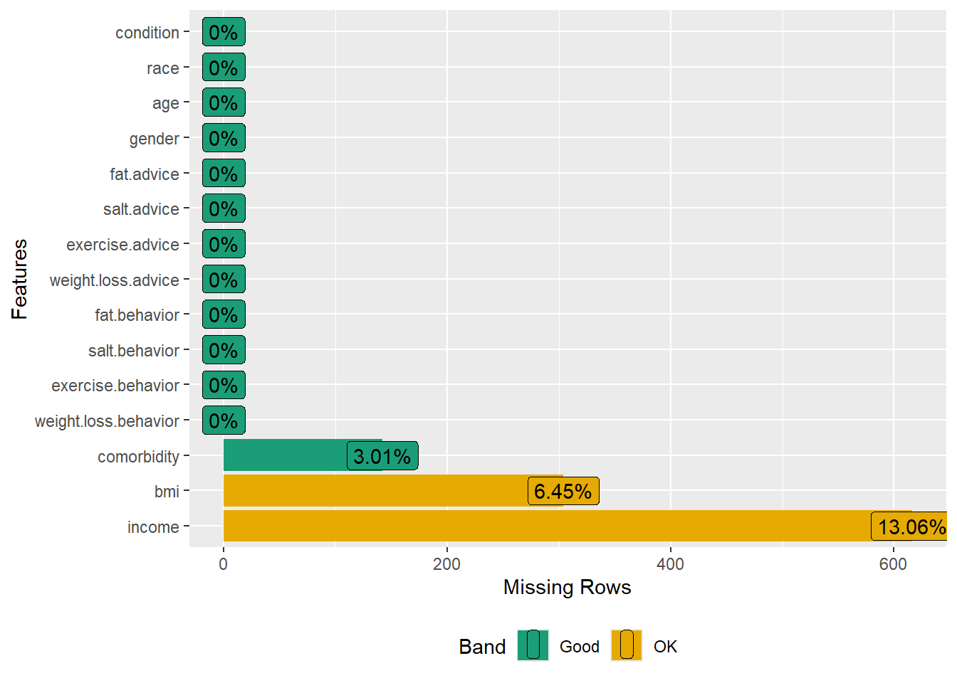
In the dataset created in 1(c), use a plot to check missingness. In the plot, include only the outcome variables, predictors, and confounders.

There are four outcome variables and four predictor variables used in the study.
The authors considered the following confounders: gender, age, income, race, bmi, condition, and comorbidity.

# 2(a) Check missingness using a plot
confounder_vars <- c("gender", "age", "income", "race", "bmi", "condition", "comorbidity")
plot_missing(dat.with.miss[, c(outcome_vars, predictor_vars, confounder_vars)])

2(b) Reproduce Table 3: Multiple imputation

Let’s we are interested in exploring the relationship between weight loss advice (exposure) and weight loss behavior (outcome). Perform multiple imputations to deal with missing values only in confounders. Use the dataset dat.with.miss.

Consider:

5 imputed datasets
10 iterations
Fit the design-adjusted logistic regression in all of the 5 imputed datasets
Obtain the pooled adjusted odds ratio with the 95% confidence intervals, i.e., create only the first column of Table 3.

You must:

Setup the data such that the variables are of appropriate types (e.g., factors, numeric). lapply function could be helpful.
Relevel the confounders as shown in Table 3.
Use the strata variable as an auxiliary variable in the imputation model, but not the survey weight or PSU variable.
There are four exposure and four outcome variables in the dataset. Include all these variables in the imputation model.
Consider predictive mean matching (pmm) method for bmi and comorbidity variable in the imputation model.
Set your seed to 123.
Remove any subject ID variable from the imputation model, if created in an intermediate step.

Hints:

The point and interval estimates could be slightly different than shown in Table 3. But they should very close.
Remember to keep count of the ineligible subjects from the full data, and consider adding them back in the imputed datasets (so that all the weight, strata and cluster information are available in the design).

# Helper Function to Reduce Duplication
# This function automates the post-analysis process for imputed data.
# It takes a 'mira' object (the result of running a model on multiple imputations)
# and returns a clean, formatted table of odds ratios and confidence intervals.
pool_and_format_results <- function(fit_mira) {
  # 'MIcombine' applies Rubin's Rules to pool the estimates from each imputed dataset.
  pooled <- MIcombine(fit_mira)
  
  # Exponentiate the log-odds coefficients and confidence intervals to get Odds Ratios (ORs).
  or_estimates <- exp(coef(pooled))
  ci_estimates <- exp(confint(pooled))
  
  # Create and return a final data frame, rounding the results for clarity.
  results_df <- data.frame(
    OR = round(or_estimates, 2),
    `2.5 %` = round(ci_estimates[, 1], 2),
    `97.5 %` = round(ci_estimates[, 2], 2)
  )
  return(results_df)
}

#----------------------------------------------------------------
# Question 2(b) Reproduce Table 3 (First Column)
#----------------------------------------------------------------

# Convert character variables to factors for regression modeling.
factor_vars <- c(outcome_vars, predictor_vars, "gender", "income", "race", "bmi", "condition")
dat.with.miss[, factor_vars] <- lapply(dat.with.miss[, factor_vars], factor)

# Set the reference levels for categorical variables to match the study's analysis.
# This ensures the odds ratios are interpreted correctly (e.g., comparing 'Female' to 'Male').
dat.with.miss <- dat.with.miss %>%
  mutate(
    gender = relevel(gender, ref = "Male"),
    income = relevel(income, ref = "400+%"),
    race = relevel(race, ref = "Non-Hispanic white"),
    condition = relevel(condition, ref = "Both")
  )

# Remove the original variables used to create 'condition' to prevent
# perfect multicollinearity during the imputation step.
dat_for_imputation <- dat.with.miss %>%
  select(-DIQ010, -BPQ020)

# Run the multiple imputation using the 'mice' package.
# m = 5: Creates 5 imputed datasets.
# maxit = 10: Runs 10 iterations for the Gibbs sampler to converge.
# meth = c(bmi = "pmm"): Specifies predictive mean matching for imputing BMI.
imputation_q2 <- mice(dat_for_imputation, m = 5, maxit = 10, seed = 123, print = FALSE,
                      meth = c(bmi = "pmm"))

# Extract the 5 imputed datasets into a single "long" format data frame.
impdata_q2 <- complete(imputation_q2, "long", include = FALSE)


# Re-integrate Ineligible Subjects for Correct Survey Variance
# This entire block is necessary to correctly estimate variance with survey data.
# The 'svydesign' object needs the full sample structure, even those outside the analysis.

# Add a flag to identify the analytic (eligible) group in the imputed data.
impdata_q2$eligible <- 1

# 1. Isolate all subjects from the original dataset who were not in our analytic sample.
dat_ineligible <- filter(dat.full, !(id %in% dat.with.miss$id))

# 2. Replicate the ineligible dataset 5 times, once for each imputation (.imp = 1 to 5).
ineligible_list <- lapply(1:5, function(i) {
  df <- dat_ineligible
  df$.imp <- i
  return(df)
})
ineligible_stacked <- do.call(rbind, ineligible_list)

# 3. Find which columns exist in the imputed data but not in the ineligible data.
cols_to_add <- setdiff(names(impdata_q2), names(ineligible_stacked))

# 4. Add these missing columns (e.g., 'condition', imputed values) to the ineligible data, filling with NA.
ineligible_stacked[, cols_to_add] <- NA

# 5. Set the eligibility flag for this group to 0.
ineligible_stacked$eligible <- 0

# 6. CRITICAL: Force the ineligible data to have the exact same column names and order
#    as the imputed data. This prevents errors when row-binding.
ineligible_final <- ineligible_stacked[, names(impdata_q2)]

# 7. Combine the imputed analytic data with the prepared ineligible data.
impdata2_full <- rbind(impdata_q2, ineligible_final)


# --- Survey Analysis --- #

# Create the complex survey design object.
# 'imputationList' tells the survey package how to handle the 5 imputed datasets.
# The design is specified on the *full* data to capture the total population structure.
design_full <- svydesign(ids = ~psu, weights = ~survey.weight, strata = ~strata,
                         data = imputationList(split(impdata2_full, impdata2_full$.imp)), nest = TRUE)

# Subset the design object to include only the eligible participants for analysis.
design_analytic <- subset(design_full, eligible == 1)

# Fit the logistic regression model across each of the 5 imputed datasets.
# 'with()' applies the 'svyglm' function to each dataset in the 'design_analytic' object.
fit_q2 <- with(design_analytic,
               svyglm(I(weight.loss.behavior == "Yes") ~ weight.loss.advice + gender + age +
                        income + race + bmi + condition + comorbidity, family = binomial("logit")))

# Use our helper function to pool the 5 models and display the final formatted results.
pool_and_format_results(fit_q2)

Question 3: Dealing with missing values in outcome, predictor, and confoudners

Perform multiple imputations to deal with missing values only in outcome, predictor, confounders. Use the Multiple Imputation then deletion (MID) approach. Use the dataset created in Subsetting according to eligibility (dat.with.miss). Consider 5 imputed datasets, 5 iterations, and fit the design-adjusted logistic regression in all of the 5 imputed datasets. Obtain the pooled adjusted odds ratio with the 95% confidence intervals. In this case, consider only one outcome and one predictor that are related to reduce fat/calories, i.e., create only the fourth column of Table 3.

Setup the data such that the variables are of appropriate types.
Relevel the confounders as shown in Table 3.
Use the strata variable as an auxiliary variable in the imputation model, but not the survey weight or PSU variable.
Include all 4 outcomes and 4 predictors in your imputation model.
Consider predictive mean matching method for bmi and comorbidity variable in the imputation model.
Set your seed to 123.
Remove any subject ID variable from the imputation model, if created in an intermediate step.
The point and interval estimates could be slightly different than shown in Table 3. But they should very close.
Remember to keep count of the ineligible subjects from the full data, and consider adding them back in the imputed datasets (so that all the weight, strata and cluster information are available in the design).

#----------------------------------------------------------------
# Question 3: Dealing with Missing Values in All Variables (MID)
#----------------------------------------------------------------

# For this question, we start with 'dat.analytic' (N=4,746), which includes
# subjects who have missing values in the outcome and predictor variables.

# STEP 1: Prepare the data for imputation.
# This involves creating the 'condition' variable and setting correct factor levels.
dat_q3_prepped <- dat.analytic %>%
  mutate(
    # Create the 'condition' variable based on diabetes and hypertension status.
    condition = case_when(
      BPQ020 == "Yes" & DIQ010 == "Yes" ~ "Both",
      DIQ010 == "Yes"                   ~ "Diabetes Only",
      BPQ020 == "Yes"                   ~ "Hypertension Only"
    ),
    # Set the reference levels for categorical variables to ensure correct interpretation of model results.
    condition = factor(condition, levels = c("Hypertension Only", "Diabetes Only", "Both")),
    gender = relevel(as.factor(gender), ref = "Male"),
    income = relevel(as.factor(income), ref = "400+%"),
    race = relevel(as.factor(race), ref = "Non-Hispanic white"),
    condition = relevel(condition, ref = "Both")
  )

# STEP 2: Convert all relevant columns to the factor data type *after* creating 'condition'.
# This avoids the "undefined columns selected" error.
factor_vars <- c(outcome_vars, predictor_vars, "gender", "income", "race", "bmi", "condition")
dat_q3_prepped[, factor_vars] <- lapply(dat_q3_prepped[, factor_vars], factor)

# STEP 3: Remove the original source variables to prevent perfect multicollinearity during imputation.
dat_for_imputation_q3 <- dat_q3_prepped %>%
  select(-DIQ010, -BPQ020)

# STEP 4: Perform multiple imputation on the prepared dataset.
# This will impute missing values in outcomes, predictors, and confounders.
imputation_q3 <- mice(dat_for_imputation_q3, m = 5, maxit = 5, seed = 123, print = FALSE,
                     meth = c(bmi = "pmm")) # Use predictive mean matching for BMI.

# Extract the 5 complete datasets into a single "long" data frame.
impdata_q3 <- complete(imputation_q3, "long", include = FALSE)


# Re-integrate Ineligible Subjects for Correct Survey Variance 
# The survey design requires the full sample structure to correctly estimate variance.

# Add an 'eligible' flag to the imputed analytic data.
impdata_q3$eligible <- 1

# Isolate subjects from the original full dataset who were not part of this analysis.
dat_ineligible_q3 <- filter(dat.full, !(id %in% dat.analytic$id))

# Replicate the ineligible dataset 5 times, one for each imputation set.
ineligible_list <- lapply(1:5, function(i) {
  df <- dat_ineligible_q3
  df$.imp <- i      # Add imputation number
  return(df)
})
ineligible_stacked <- do.call(rbind, ineligible_list)

# Align the structure of the ineligible data to perfectly match the imputed data.
cols_to_add <- setdiff(names(impdata_q3), names(ineligible_stacked))
ineligible_stacked[, cols_to_add] <- NA # Add missing columns (e.g., 'condition', '.id') as NA.
ineligible_stacked$eligible <- 0         # Set eligibility flag for this group.

# CRITICAL: Reorder columns to prevent 'rbind' errors.
ineligible_final <- ineligible_stacked[, names(impdata_q3)]

# Combine the imputed analytic data and the prepared ineligible data.
impdata3_full <- rbind(impdata_q3, ineligible_final)


# --- Survey Analysis using Multiple Imputation then Deletion (MID) --- #

# Create the complex survey design object on the full combined data.
design_full_q3 <- svydesign(ids = ~psu, weights = ~survey.weight, strata = ~strata,
                         data = imputationList(split(impdata3_full, impdata3_full$.imp)), nest = TRUE)

# Apply the "Deletion" step of MID: subset the design to the analytic group
# AND only those with complete data for the specific variables in this model.
design_analytic_q3 <- subset(design_full_q3, eligible == 1 & complete.cases(fat.behavior, fat.advice))

# Fit the logistic regression model across each of the 5 imputed datasets.
fit_q3 <- with(design_analytic_q3,
               svyglm(I(fat.behavior == "Yes") ~ fat.advice + gender + age + income +
                        race + bmi + condition + comorbidity, family = binomial("logit")))

# Use our helper function to pool the results and display the final formatted table.
pool_and_format_results(fit_q3)