Collinear predictors
In this tutorial, we’ll continue with the data analysis. We’ll focus on an analysis of an NHANES data. This data contains over 1200 observations and 33 variables. These variables come in various types: numeric, categorical, and binary. Our primary goal is to fit a linear regression model to predict cholesterol levels.
Load data
Let us load the dataset and see structure of the variables:
load(file = "Data/predictivefactors/cholesterolNHANES15.RData")
#head(analytic)
str(analytic)
#> 'data.frame':    1267 obs. of  33 variables:
#>  $ ID                   : num  83732 83733 83741 83747 83750 ...
#>  $ gender               : chr  "Male" "Male" "Male" "Male" ...
#>  $ age                  : num  62 53 22 46 45 30 60 69 24 70 ...
#>  $ born                 : chr  "Born in 50 US states or Washingt" "Others" "Born in 50 US states or Washingt" "Others" ...
#>  $ race                 : chr  "White" "White" "Black" "White" ...
#>  $ education            : chr  "College" "High.School" "College" "College" ...
#>  $ married              : chr  "Married" "Previously.married" "Never.married" "Married" ...
#>  $ income               : chr  "Between.55kto99k" "<25k" "Between.25kto54k" "<25k" ...
#>  $ weight               : num  135630 25282 39353 35674 97002 ...
#>  $ psu                  : num  1 1 2 1 1 1 1 2 1 2 ...
#>  $ strata               : num  125 125 128 121 125 124 128 120 130 132 ...
#>  $ diastolicBP          : num  70 88 70 94 70 50 74 70 72 54 ...
#>  $ systolicBP           : num  128 146 110 144 116 104 142 146 126 144 ...
#>  $ bodyweight           : num  94.8 90.4 76.6 86.2 76.2 71.2 75.6 84 89.2 81.7 ...
#>  $ bodyheight           : num  184 171 165 177 178 ...
#>  $ bmi                  : num  27.8 30.8 28 27.6 24.1 26.6 35.9 31 26.9 27 ...
#>  $ waist                : num  101.1 107.9 86.6 104.3 90.1 ...
#>  $ smoke                : chr  "Not.at.all" "Every.day" "Some.days" "Every.day" ...
#>  $ alcohol              : num  1 6 8 1 3 2 1 1 2 2 ...
#>  $ cholesterol          : num  173 265 164 242 181 184 205 287 126 192 ...
#>  $ cholesterolM2        : num  4.47 6.85 4.24 6.26 4.68 4.76 5.3 7.42 3.26 4.97 ...
#>  $ triglycerides        : num  158 170 77 497 63 62 169 245 95 64 ...
#>  $ uric.acid            : num  4.2 7 6 6.5 5.4 5.5 5.1 4.3 7.6 7.1 ...
#>  $ protein              : num  7.5 7.4 7.4 6.8 7.4 6.7 7.4 6.8 7.3 7.2 ...
#>  $ bilirubin            : num  0.5 0.6 0.2 0.5 0.7 0.8 0.4 0.6 1.2 1.2 ...
#>  $ phosphorus           : num  4.7 4.4 5.3 3.6 3.9 3.4 3.9 4.4 3.2 3 ...
#>  $ sodium               : num  136 140 139 138 138 136 139 140 140 139 ...
#>  $ potassium            : num  4.3 4.55 4.16 4.27 3.91 3.97 3.99 4.25 3.8 4.63 ...
#>  $ globulin             : num  2.9 2.9 3 2.6 2.8 2.5 3.2 2.3 2.7 2.6 ...
#>  $ calcium              : num  9.8 9.8 9.3 9.3 9.3 9.4 9.6 9.6 9.6 9.6 ...
#>  $ physical.work        : chr  "No" "No" "No" "No" ...
#>  $ physical.recreational: chr  "No" "No" "Yes" "No" ...
#>  $ diabetes             : chr  "Yes" "No" "No" "No" ...
#>  - attr(*, "na.action")= 'omit' Named int [1:3739] 3 4 5 6 8 9 13 14 15 16 ...
#>   ..- attr(*, "names")= chr [1:3739] "3" "4" "5" "6" ...
Describe the data
require(rms)
describe(analytic)
#> analytic
#>
#>  33  Variables      1267  Observations
#> --------------------------------------------------------------------------------
#> ID
#>        n  missing distinct     Info     Mean  pMedian      Gmd      .05
#>     1267        0     1267        1    88660    88660     3366    84250
#>      .10      .25      .50      .75      .90      .95
#>    84687    86019    88692    91252    92670    93089
#>
#> lowest : 83732 83733 83741 83747 83750, highest: 93617 93633 93643 93659 93685
#> --------------------------------------------------------------------------------
#> gender
#>        n  missing distinct
#>     1267        0        2
#>
#> Value      Female   Male
#> Frequency     496    771
#> Proportion  0.391  0.609
#> --------------------------------------------------------------------------------
#> age
#>        n  missing distinct     Info     Mean  pMedian      Gmd      .05
#>     1267        0       61        1    49.91       50    19.18       24
#>      .10      .25      .50      .75      .90      .95
#>       27       36       51       63       72       78
#>
#> lowest : 20 21 22 23 24, highest: 76 77 78 79 80
#> --------------------------------------------------------------------------------
#> born
#>        n  missing distinct
#>     1267        0        2
#>
#> Value      Born in 50 US states or Washingt                           Others
#> Frequency                               991                              276
#> Proportion                            0.782                            0.218
#> --------------------------------------------------------------------------------
#> race
#>        n  missing distinct
#>     1267        0        4
#>
#> Value         Black Hispanic    Other    White
#> Frequency       246      337      132      552
#> Proportion    0.194    0.266    0.104    0.436
#> --------------------------------------------------------------------------------
#> education
#>        n  missing distinct
#>     1267        0        3
#>
#> Value          College High.School      School
#> Frequency          648         523          96
#> Proportion       0.511       0.413       0.076
#> --------------------------------------------------------------------------------
#> married
#>        n  missing distinct
#>     1267        0        3
#>
#> Value                 Married      Never.married Previously.married
#> Frequency                 751                226                290
#> Proportion              0.593              0.178              0.229
#> --------------------------------------------------------------------------------
#> income
#>        n  missing distinct
#>     1267        0        4
#>
#> Value                  <25k Between.25kto54k Between.55kto99k         Over100k
#> Frequency               344              435              297              191
#> Proportion            0.272            0.343            0.234            0.151
#> --------------------------------------------------------------------------------
#> weight
#>        n  missing distinct     Info     Mean  pMedian      Gmd      .05
#>     1267        0     1184        1    48904    38496    44337     9158
#>      .10      .25      .50      .75      .90      .95
#>    11549    19540    30335    63822   121803   151546
#>
#> lowest : 5470.04 5948.95 6197.66 6480.95 6703.84
#> highest: 203563  207197  213611  218139  224892
#> --------------------------------------------------------------------------------
#> psu
#>        n  missing distinct     Info     Mean
#>     1267        0        2     0.75    1.493
#>
#> Value          1     2
#> Frequency    642   625
#> Proportion 0.507 0.493
#> --------------------------------------------------------------------------------
#> strata
#>        n  missing distinct     Info     Mean  pMedian      Gmd      .05
#>     1267        0       15    0.994    126.3      126    4.792      120
#>      .10      .25      .50      .75      .90      .95
#>      121      123      126      130      132      133
#>
#> Value        119   120   121   122   123   124   125   126   127   128   129
#> Frequency     47    74   118    63    77    66   114   104   107    65    53
#> Proportion 0.037 0.058 0.093 0.050 0.061 0.052 0.090 0.082 0.084 0.051 0.042
#>
#> Value        130   131   132   133
#> Frequency     99   120    95    65
#> Proportion 0.078 0.095 0.075 0.051
#>
#> For the frequency table, variable is rounded to the nearest 0
#> --------------------------------------------------------------------------------
#> diastolicBP
#>        n  missing distinct     Info     Mean  pMedian      Gmd      .05
#>     1267        0       41    0.997    70.37       70    13.99       52
#>      .10      .25      .50      .75      .90      .95
#>       54       62       70       78       86       92
#>
#> lowest :   0  26  34  38  40, highest: 104 106 108 110 112
#> --------------------------------------------------------------------------------
#> systolicBP
#>        n  missing distinct     Info     Mean  pMedian      Gmd      .05
#>     1267        0       56    0.998    126.5      125     19.3    102.0
#>      .10      .25      .50      .75      .90      .95
#>    106.0    114.0    124.0    136.0    148.8    160.0
#>
#> lowest :  84  88  90  92  94, highest: 194 196 206 218 236
#> --------------------------------------------------------------------------------
#> bodyweight
#>        n  missing distinct     Info     Mean  pMedian      Gmd      .05
#>     1267        0      615        1    84.95    83.15    23.56    56.29
#>      .10      .25      .50      .75      .90      .95
#>    61.10    69.70    81.40    97.00   113.44   127.47
#>
#> lowest : 39.7  39.8  40.7  42.6  42.7 , highest: 161.9 166.3 175.7 175.9 178.4
#> --------------------------------------------------------------------------------
#> bodyheight
#>        n  missing distinct     Info     Mean  pMedian      Gmd      .05
#>     1267        0      376        1    169.2    169.2    10.66    153.8
#>      .10      .25      .50      .75      .90      .95
#>    157.0    162.6    169.3    176.2    181.1    184.2
#>
#> lowest : 143.8 144.2 145.2 145.9 146.2, highest: 194.6 195.1 195.6 198.4 201
#> --------------------------------------------------------------------------------
#> bmi
#>        n  missing distinct     Info     Mean  pMedian      Gmd      .05
#>     1267        0      284        1    29.58       29    7.403    20.60
#>      .10      .25      .50      .75      .90      .95
#>    22.06    24.80    28.60    33.30    38.24    42.00
#>
#> lowest : 16.3 17.5 17.6 17.7 17.9, highest: 57.2 57.6 59.4 60.7 64.5
#> --------------------------------------------------------------------------------
#> waist
#>        n  missing distinct     Info     Mean  pMedian      Gmd      .05
#>     1267        0      544        1    101.8      101    18.47     77.1
#>      .10      .25      .50      .75      .90      .95
#>     81.4     90.5    100.3    111.2    122.8    132.5
#>
#> lowest : 65    65.5  66.5  68.2  68.7 , highest: 159.2 159.8 160.2 160.5 161.5
#> --------------------------------------------------------------------------------
#> smoke
#>        n  missing distinct
#>     1267        0        3
#>
#> Value       Every.day Not.at.all  Some.days
#> Frequency         448        665        154
#> Proportion      0.354      0.525      0.122
#> --------------------------------------------------------------------------------
#> alcohol
#>        n  missing distinct     Info     Mean  pMedian      Gmd      .05
#>     1267        0       14    0.952    3.109      2.5    2.419        1
#>      .10      .25      .50      .75      .90      .95
#>        1        1        2        4        6        8
#>
#> Value          1     2     3     4     5     6     7     8     9    10    11
#> Frequency    336   371   189   106    79    95    10    26     4    20     1
#> Proportion 0.265 0.293 0.149 0.084 0.062 0.075 0.008 0.021 0.003 0.016 0.001
#>
#> Value         12    14    15
#> Frequency     23     1     6
#> Proportion 0.018 0.001 0.005
#>
#> For the frequency table, variable is rounded to the nearest 0
#> --------------------------------------------------------------------------------
#> cholesterol
#>        n  missing distinct     Info     Mean  pMedian      Gmd      .05
#>     1267        0      203        1    193.1      191    47.47    132.0
#>      .10      .25      .50      .75      .90      .95
#>    142.0    162.5    191.0    217.0    248.0    268.0
#>
#> lowest :  81  93  97 100 101, highest: 345 348 349 358 545
#> --------------------------------------------------------------------------------
#> cholesterolM2
#>        n  missing distinct     Info     Mean  pMedian      Gmd      .05
#>     1267        0      203        1    4.994     4.94    1.228    3.410
#>      .10      .25      .50      .75      .90      .95
#>    3.670    4.205    4.940    5.610    6.410    6.930
#>
#> lowest : 2.09  2.4   2.51  2.59  2.61 , highest: 8.92  9     9.03  9.26  14.09
#> --------------------------------------------------------------------------------
#> triglycerides
#>        n  missing distinct     Info     Mean  pMedian      Gmd      .05
#>     1267        0      361        1    165.8    141.5    124.1     48.0
#>      .10      .25      .50      .75      .90      .95
#>     59.0     84.0    127.0    201.5    309.0    396.6
#>
#> lowest :   18   21   24   25   31, highest:  964 1020 1157 1253 3061
#> --------------------------------------------------------------------------------
#> uric.acid
#>        n  missing distinct     Info     Mean  pMedian      Gmd      .05
#>     1267        0       84        1    5.598     5.55    1.626     3.43
#>      .10      .25      .50      .75      .90      .95
#>     3.80     4.60     5.50     6.50     7.40     8.00
#>
#> lowest : 1.6  2.2  2.3  2.4  2.5 , highest: 10.2 10.3 11.7 12.2 18
#> --------------------------------------------------------------------------------
#> protein
#>        n  missing distinct     Info     Mean  pMedian      Gmd      .05
#>     1267        0       32    0.995    7.126      7.1   0.5095      6.4
#>      .10      .25      .50      .75      .90      .95
#>      6.6      6.8      7.1      7.4      7.7      7.9
#>
#> lowest : 5.7 5.8 5.9 6   6.1, highest: 8.4 8.5 8.6 8.8 9
#> --------------------------------------------------------------------------------
#> bilirubin
#>        n  missing distinct     Info     Mean  pMedian      Gmd      .05
#>     1267        0       31    0.984   0.5467      0.5   0.2949      0.2
#>      .10      .25      .50      .75      .90      .95
#>      0.2      0.4      0.5      0.7      0.9      1.0
#>
#> lowest : 0    0.01 0.02 0.03 0.04, highest: 1.8  2    2.1  2.6  3.3
#> --------------------------------------------------------------------------------
#> phosphorus
#>        n  missing distinct     Info     Mean  pMedian      Gmd      .05
#>     1267        0       37    0.996    3.642     3.65    0.593      2.8
#>      .10      .25      .50      .75      .90      .95
#>      3.0      3.3      3.6      4.0      4.3      4.5
#>
#> lowest : 1.8 2   2.2 2.3 2.4, highest: 5.2 5.3 5.4 5.6 6.1
#> --------------------------------------------------------------------------------
#> sodium
#>        n  missing distinct     Info     Mean  pMedian      Gmd      .05
#>     1267        0       20    0.977    138.5    138.5    2.383      135
#>      .10      .25      .50      .75      .90      .95
#>      136      137      139      140      141      142
#>
#> Value        124   126   129   130   131   132   133   134   135   136   137
#> Frequency      1     1     1     1     5     4    11    23    46    93   176
#> Proportion 0.001 0.001 0.001 0.001 0.004 0.003 0.009 0.018 0.036 0.073 0.139
#>
#> Value        138   139   140   141   142   143   144   146   148
#> Frequency    235   260   206   112    55    29     6     1     1
#> Proportion 0.185 0.205 0.163 0.088 0.043 0.023 0.005 0.001 0.001
#>
#> For the frequency table, variable is rounded to the nearest 0
#> --------------------------------------------------------------------------------
#> potassium
#>        n  missing distinct     Info     Mean  pMedian      Gmd      .05
#>     1267        0      175        1    3.985     3.98   0.3725     3.45
#>      .10      .25      .50      .75      .90      .95
#>     3.57     3.78     3.98     4.19     4.40     4.54
#>
#> lowest : 2.6  2.92 2.96 3.07 3.09, highest: 5.15 5.21 5.36 5.37 5.51
#> --------------------------------------------------------------------------------
#> globulin
#>        n  missing distinct     Info     Mean  pMedian      Gmd      .05
#>     1267        0       29    0.994    2.799      2.8   0.4536      2.2
#>      .10      .25      .50      .75      .90      .95
#>      2.3      2.5      2.8      3.0      3.3      3.5
#>
#> lowest : 1.6 1.8 1.9 2   2.1, highest: 4.1 4.2 4.3 4.5 5.5
#> --------------------------------------------------------------------------------
#> calcium
#>        n  missing distinct     Info     Mean  pMedian      Gmd      .05
#>     1267        0       25    0.991    9.335     9.35   0.3786      8.8
#>      .10      .25      .50      .75      .90      .95
#>      8.9      9.1      9.3      9.6      9.7      9.9
#>
#> lowest : 8.4  8.5  8.6  8.7  8.8 , highest: 10.4 10.5 10.7 11   11.1
#> --------------------------------------------------------------------------------
#> physical.work
#>        n  missing distinct
#>     1267        0        2
#>
#> Value         No   Yes
#> Frequency    895   372
#> Proportion 0.706 0.294
#> --------------------------------------------------------------------------------
#> physical.recreational
#>        n  missing distinct
#>     1267        0        2
#>
#> Value         No   Yes
#> Frequency   1002   265
#> Proportion 0.791 0.209
#> --------------------------------------------------------------------------------
#> diabetes
#>        n  missing distinct
#>     1267        0        2
#>
#> Value        No  Yes
#> Frequency  1064  203
#> Proportion 0.84 0.16
#> --------------------------------------------------------------------------------
Collinearity
Avoiding collinear variables can result in a more interpretable, stable, and efficient predictive model. Collinearity refers to a situation in which two or more predictor variables in a multiple regression model are highly correlated, meaning that one can be linearly predicted from the others with substantial accuracy. Collinearity poses several issues for predictive analysis:
Reduced Interpretability: When predictor variables are highly correlated, it becomes challenging to isolate the impact of individual predictors on the response variable. In other words, it is difficult to determine which predictor is genuinely influential in explaining variance in the response variable. This reduces the interpretability of the model.
Unstable Coefficients: Collinearity can lead to inflated standard errors of the regression coefficients. This means that the coefficients can be very sensitive to small changes in the data, making the model unstable and less generalizable to new, unseen data.
Overfitting: When predictors are collinear, the model is more likely to fit to the noise in the data rather than the actual signal. This is a manifestation of overfitting, where the model becomes too complex and captures random noise. Overfitted models will perform poorly on new, unseen data.
Inefficiency: Including redundant variables (collinear variables) does not add additional information to the model. This could be inefficient, especially when dealing with large datasets, as it increases computational costs without improving model performance.
Multicollinearity Diagnostics
Several techniques are available for diagnosing multicollinearity, including:
Variance Inflation Factor (VIF): The VIF is a measure of multicollinearity, which measures how much the variance of a regression coefficient is increased because of multicollinearity. A general rule of thumb is that if VIF exceeds 4 or 5, multicollinearity is present.
Eigenvalues and Eigenvectors of the correlation/covariance matrix: The eigenvalues of the correlation matrix can also be used to measure the presence of multicollinearity, with one or more eigenvalues close to zero indicating multicollinearity.
Pairwise correlation matrices: Large correlation coefficients in the correlation matrix of predictors indicate the possibility of multicollinearity.
Remedies
Some common ways to handle collinearity include:
- Removing one of the correlated predictors
- Combining correlated predictors into a single composite predictor
- Using regularization techniques like Ridge Regression, which can help handle collinearity by adding a penalty term. Ridge regression adds a small amount of bias to the regression estimates, which in turn reduces the standard error, addresses the collinearity issue to some extent, and makes the results more reliable.
Identify collinear predictors
We can also use hclust and varclus or variable clustering, i.e., to identify collinear predictors
hclust is the hierarchical clustering function where default is squared Spearman correlation coefficients to detect monotonic but nonlinear relationships.
require(Hmisc)
sel.names <- c("gender", "age", "born", "race", "education",
               "married", "income", "diastolicBP", "systolicBP",
               "bodyweight", "bodyheight", "bmi", "waist", "smoke",
               "alcohol",  "cholesterol", "triglycerides",
               "uric.acid", "protein", "bilirubin", "phosphorus",
               "sodium", "potassium", "globulin", "calcium",
               "physical.work", "physical.recreational",
               "diabetes")
var.cluster <- varclus(~., data = analytic[sel.names])
# var.cluster
plot(var.cluster)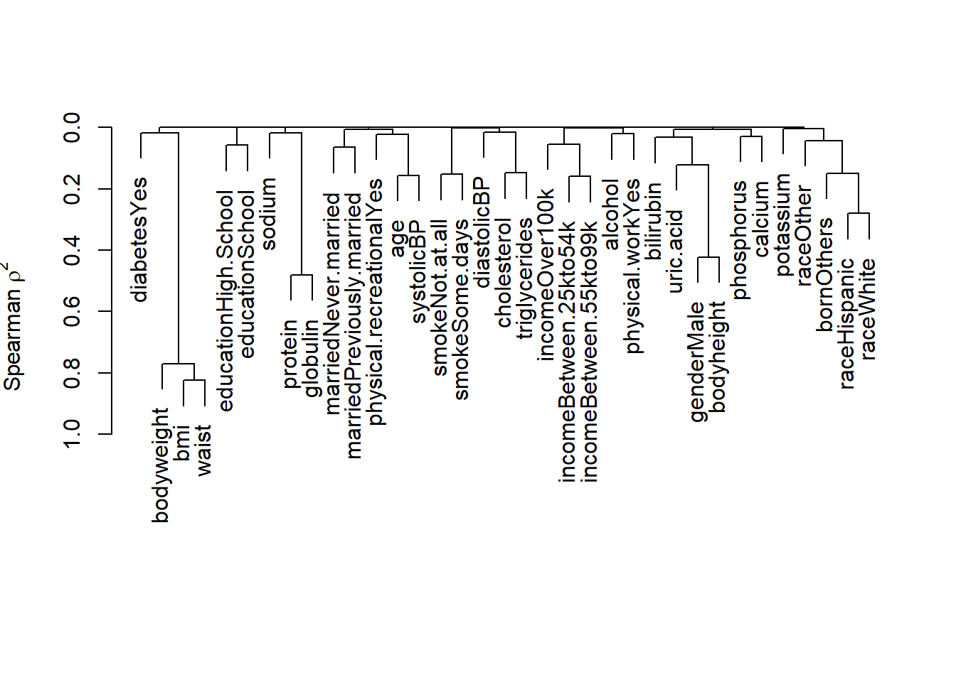
In this plot, Spearman correlation or Spearman’s \(\rho\)(rho) assesses the monotonic but nonlinear relationships predictors. We can also specify linear relationships such as Pearson correlation. A high correlation coefficient indicates predictors are highly correlated. For example, Spearman’s \(\rho\) is more than 0.8 for bodyweight, BMI, and waist, indicating high collinearity between these predictors.
Video content (optional)
For those who prefer a video walkthrough, feel free to watch the video below, which offers a description of an earlier version of the above content.