Comparing results

In this tutorial, we will use the RHC dataset in exploring the relationship between RHC (yes/no) and death (yes/no). We will use the following approaches:

logistic regression
propensity score matching and weighting with logistic regression
propensity score matching and weighting with Super Learner
TMLE

Load packages

We load several R packages required for fitting the models.

# Load required packages
library(tableone)
library(Publish)
library(randomForest)
library(tmle)
library(xgboost)
library(kableExtra)
library(SuperLearner)
library(dbarts)
library(MatchIt)
library(cobalt)
library(survey)
library(knitr)

Load dataset

load(file = "Data/machinelearningCausal/cl2.RData")
ls()
#> [1] "baselinevars"    "has_annotations" "ObsData"         "tab0"

# Data
dat <- ObsData
head(dat)


# Data dimension
dim(dat)
#> [1] 5735   52

Confounder list in the baselinevars vector is

Confounders
Disease.category
Cancer
Cardiovascular
Congestive.HF
Dementia
Psychiatric
Pulmonary
Renal
Hepatic
GI.Bleed
Tumor
Immunosupperssion
Transfer.hx
MI
age
sex
edu
DASIndex
APACHE.score
Glasgow.Coma.Score
blood.pressure
WBC
Heart.rate
Respiratory.rate
Temperature
PaO2vs.FIO2
Albumin
Hematocrit
Bilirubin
Creatinine
Sodium
Potassium
PaCo2
PH
Weight
DNR.status
Medical.insurance
Respiratory.Diag
Cardiovascular.Diag
Neurological.Diag
Gastrointestinal.Diag
Renal.Diag
Metabolic.Diag
Hematologic.Diag
Sepsis.Diag
Trauma.Diag
Orthopedic.Diag
race
income

Logistic regression

Let us define the regression formula and fit logistic regression, adjusting for baseline confounders.

# Formula
Formula <- formula(paste("Death ~ RHC.use + ", 
                         paste(baselinevars, 
                               collapse = " + ")))

# Logistic regression
fit.glm <- glm(Formula, 
               data = dat, 
               family = binomial)

We can use flextable package to view fit.glm, the regression output:

Variable	Odds_Ratio	CI_Lower	CI_Upper
RHC.use	1.42	1.23	1.65

As we can see, the odds of death was 42% higher among those participants with RHC use than those with no RHC use.

Propensity score matching with logistic regression

Now we will use propensity score matching, where propensity score will be estimated using logistic regression. The first step is to define the propensity score formula and estimate the propensity scores.

Step 1

# Propensity score model define
ps.formula <- as.formula(paste0("RHC.use ~ ", 
                                paste(baselinevars, 
                                      collapse = "+")))

# Propensity score model fitting
fit.ps <- glm(ps.formula, 
              data = dat, 
              family = binomial)

# Propensity scores
dat$ps <- predict(fit.ps, 
                  type = "response")
summary(dat$ps)
#>     Min.  1st Qu.   Median     Mean  3rd Qu.     Max. 
#> 0.002478 0.161446 0.358300 0.380819 0.574319 0.968425

Step 2

The second step is to match exposed (i.e., RHC users) to unexposed (i.e., RHC non-users) based on the propensity scores. We will use nearest neighborhood and caliper approach.

# Caliper
caliper <- 0.2*sd(log(dat$ps/(1-dat$ps)))

# 1:1 matching
set.seed(123)
match.obj <- matchit(ps.formula, 
                     data = dat,
                     distance = dat$ps, 
                     method = "nearest",
                     ratio = 1,
                     caliper = caliper)

# See how many matched
match.obj 
#> A matchit object
#>  - method: 1:1 nearest neighbor matching without replacement
#>  - distance: User-defined [caliper]
#>  - caliper: <distance> (0.068)
#>  - number of obs.: 5735 (original), 3478 (matched)
#>  - target estimand: ATT
#>  - covariates: too many to name

# Extract matched data
matched.data <- match.data(match.obj)

# Overlap checking
bal.plot(match.obj,
         var.name="distance",
         which="both",
         type = "density",
         colors = c("red","blue"))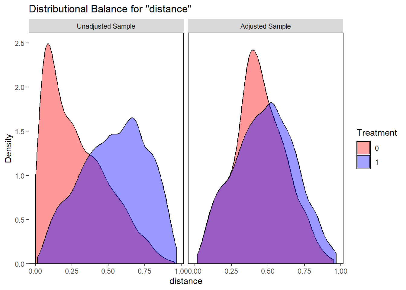

Step 3

The third step is to check the balancing on the matched data. We will compare the similarity of baseline characteristics between RHC users and non-users in the propensity score matched sample. Let’s consider SMD >0.1 as imbalanced.

# Balance checking in terms of SMD - using love plot
love.plot(match.obj, 
          binary = "std", 
          grid = TRUE,
          thresholds = c(m = .1),
          colors = c("red","blue"))


# Balance checking in terms of SMD - using tableone
tab1b <- CreateTableOne(vars = baselinevars, strata = "RHC.use", 
                        data = matched.data, includeNA = T,
                        addOverall = F, test = F)
#print(tab1b, showAllLevels = T, catDigits = 2, smd = T)

ExtractSmd(tab1b) shows

Variables	1 vs 2
Disease.category	0.06
Cancer	0.03
Cardiovascular	0.03
Congestive.HF	0.00
Dementia	0.01
Psychiatric	0.04
Pulmonary	0.04
Renal	0.03
Hepatic	0.01
GI.Bleed	0.00
Tumor	0.01
Immunosupperssion	0.01
Transfer.hx	0.03
MI	0.01
age	0.04
sex	0.02
edu	0.03
DASIndex	0.03
APACHE.score	0.08
Glasgow.Coma.Score	0.01
blood.pressure	0.07
WBC	0.01
Heart.rate	0.00
Respiratory.rate	0.04
Temperature	0.02
PaO2vs.FIO2	0.06
Albumin	0.03
Hematocrit	0.03
Bilirubin	0.03
Creatinine	0.03
Sodium	0.02
Potassium	0.01
PaCo2	0.04
PH	0.02
Weight	0.02
DNR.status	0.00
Medical.insurance	0.06
Respiratory.Diag	0.06
Cardiovascular.Diag	0.05
Neurological.Diag	0.04
Gastrointestinal.Diag	0.01
Renal.Diag	0.02
Metabolic.Diag	0.01
Hematologic.Diag	0.01
Sepsis.Diag	0.03
Trauma.Diag	0.02
Orthopedic.Diag	0.05
race	0.02
income	0.06

After propensity score matching, all the confounders are balanced in terms of SMD. Now, we will fit the outcome model on the matched data.

Step 4

fit.psm <- glm(Death ~ RHC.use, 
               data = matched.data, 
               family = binomial)

Summary of fit.psm:

Variable	Odds_Ratio	CI_Lower	CI_Upper
RHC.use	1.29	1.12	1.48

In the propensity score matched data, the odds of death was 29% higher among those participants with RHC use than those with no RHC use.

Propensity score weighting with logistic regression

Now we will use the propensity score weighting approach where propensity scores are estimated using logistic regression.

Step 1

Step 1 is the same as we did it for the propensity score matching.

Step 2

For the second step, we will calculate the stabilized inverse probability weight.

dat$ipw <- with(dat, ifelse(RHC.use==1, mean(RHC.use)/ps, 
                            mean(1-RHC.use)/(1-ps)))
summary(dat$ipw)
#>    Min. 1st Qu.  Median    Mean 3rd Qu.    Max. 
#>  0.3932  0.6571  0.7781  0.9953  1.0624 24.1854

Step 3

Now, we will check the balance in terms of SMD.

# Design with inverse probability weights
w.design <- svydesign(id = ~1, weights = ~ipw, data = dat, nest = F)

# Balance checking in terms of SMD
tab1e <- svyCreateTableOne(vars = baselinevars, strata = "RHC.use", 
                           data = w.design, includeNA = T, 
                           addOverall = F, test = F)
#print(tab1e, showAllLevels = T, catDigits = 2, smd = T)

ExtractSmd(tab1e) shows

Variables	1 vs 2
Disease.category	0.02
Cancer	0.01
Cardiovascular	0.01
Congestive.HF	0.00
Dementia	0.05
Psychiatric	0.02
Pulmonary	0.02
Renal	0.01
Hepatic	0.00
GI.Bleed	0.02
Tumor	0.00
Immunosupperssion	0.01
Transfer.hx	0.01
MI	0.00
age	0.05
sex	0.03
edu	0.00
DASIndex	0.04
APACHE.score	0.01
Glasgow.Coma.Score	0.00
blood.pressure	0.01
WBC	0.04
Heart.rate	0.02
Respiratory.rate	0.00
Temperature	0.01
PaO2vs.FIO2	0.00
Albumin	0.03
Hematocrit	0.02
Bilirubin	0.01
Creatinine	0.01
Sodium	0.01
Potassium	0.03
PaCo2	0.02
PH	0.01
Weight	0.02
DNR.status	0.04
Medical.insurance	0.03
Respiratory.Diag	0.01
Cardiovascular.Diag	0.01
Neurological.Diag	0.01
Gastrointestinal.Diag	0.01
Renal.Diag	0.01
Metabolic.Diag	0.00
Hematologic.Diag	0.00
Sepsis.Diag	0.01
Trauma.Diag	0.01
Orthopedic.Diag	0.01
race	0.02
income	0.02

All confounders are balanced (SMD < 0.1).

Step 4

fit.ipw <- svyglm(Death ~ RHC.use, 
                  design = w.design, 
                  family = binomial)

Summary of fit.ipw:

Variable	Odds_Ratio	CI_Lower	CI_Upper
RHC.use	1.30	1.11	1.53

In the propensity score weighted data, the odds of death was 30% higher among those participants with RHC use than those with no RHC use.

Propensity score matching with super learner

Now we will use the propensity score matching, where we will be using super learner to calculate the propensity scores. We use logistic, LASSO, and XGBoost as the candidate learners.

Step 1

set.seed(123)
ps.fit <- CV.SuperLearner(
  Y = dat$RHC.use,
  X = dat[,baselinevars], 
  family = "binomial",
  SL.library = c("SL.glm", "SL.glmnet", "SL.xgboost"), 
  verbose = FALSE,
  V = 5, 
  method = "method.NNLS")

# Propensity scores for all learners  
predictions <- cbind(ps.fit$SL.predict, ps.fit$library.predict)
head(predictions)
#>                SL.glm_All SL.glmnet_All SL.xgboost_All
#> [1,] 0.3632635 0.39789364    0.39569431     0.32144672
#> [2,] 0.5870492 0.64983590    0.61497078     0.54465985
#> [3,] 0.5740246 0.66329951    0.65396650     0.46847290
#> [4,] 0.2172501 0.33044244    0.34478278     0.02363573
#> [5,] 0.6347749 0.45972157    0.43779434     0.86645132
#> [6,] 0.0272532 0.03420477    0.03629319     0.01730520

# Propensity scores for super learner
dat$ps.sl <- predictions[,1]
summary(dat$ps.sl)
#>     Min.  1st Qu.   Median     Mean  3rd Qu.     Max. 
#> 0.001671 0.147762 0.337664 0.376282 0.587237 0.975584

Step 2

The same as before, we will match exposed to unexposed based on their propensity scores.

# Caliper
caliper <- 0.2*sd(log(dat$ps.sl/(1-dat$ps.sl)))

# 1:1 matching
set.seed(123)
match.obj2 <- matchit(ps.formula, 
                      data = dat,
                      distance = dat$ps.sl, 
                      method = "nearest",
                      ratio = 1,
                      caliper = caliper)

# See how many matched
match.obj2 
#> A matchit object
#>  - method: 1:1 nearest neighbor matching without replacement
#>  - distance: User-defined [caliper]
#>  - caliper: <distance> (0.075)
#>  - number of obs.: 5735 (original), 3430 (matched)
#>  - target estimand: ATT
#>  - covariates: too many to name

# Extract matched data
matched.data.sl <- match.data(match.obj2) 

# Overlap checking
bal.plot(match.obj2,
         var.name="distance",
         which="both",
         type = "density",
         colors = c("red","blue"))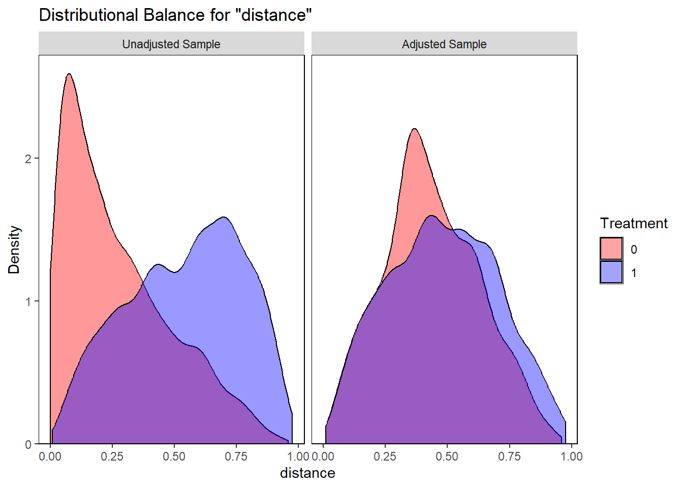

Step 3

Now we will check the balancing on the matched data.

# Balance checking in terms of SMD - using love plot
love.plot(match.obj2, 
          binary = "std", 
          grid = TRUE,
          thresholds = c(m = .1),
          colors = c("red","blue"))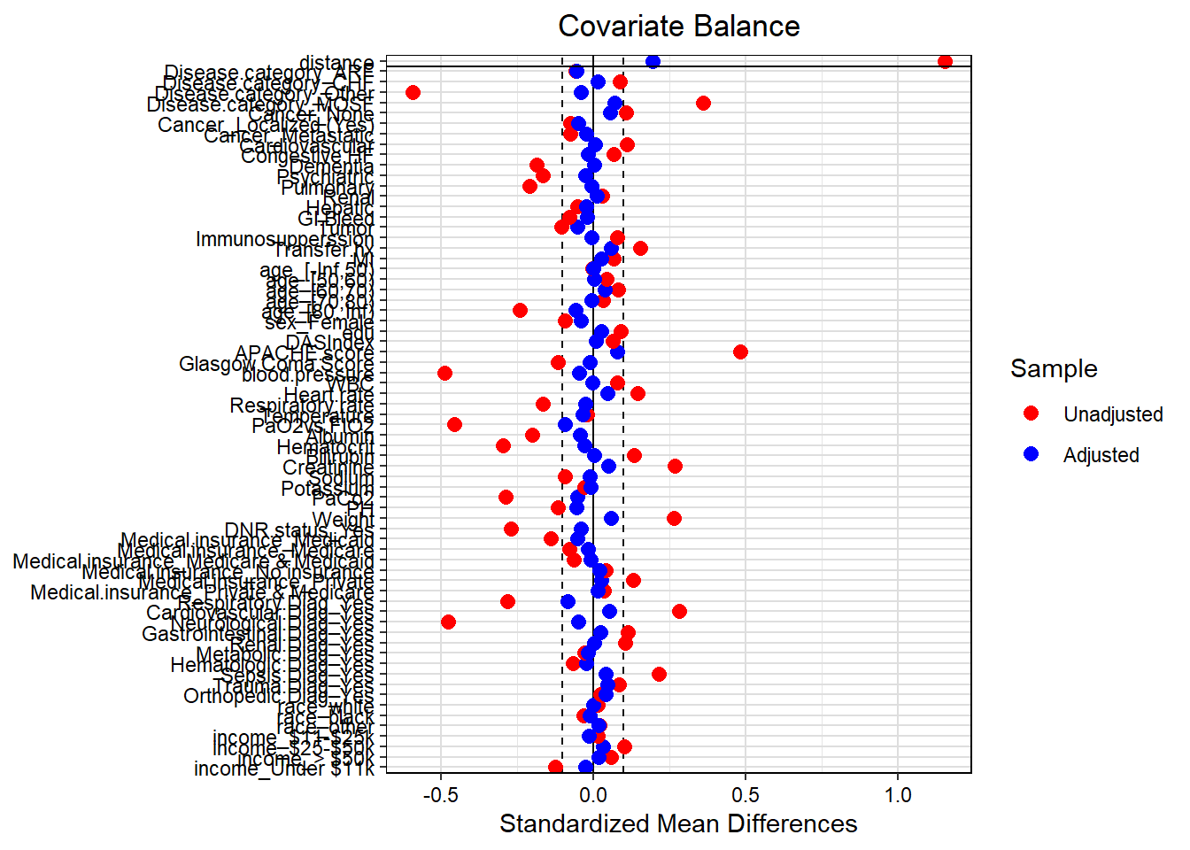


# Balance checking in terms of SMD - using tableone
tab1c <- CreateTableOne(vars = baselinevars, strata = "RHC.use", 
                        data = matched.data.sl, includeNA = T, 
                        addOverall = T, test = F)
#print(tab1c, showAllLevels = T, catDigits = 2, smd = T)

ExtractSmd(tab1c) shows

Variables	1 vs 2
Disease.category	0.08
Cancer	0.05
Cardiovascular	0.01
Congestive.HF	0.02
Dementia	0.00
Psychiatric	0.02
Pulmonary	0.01
Renal	0.01
Hepatic	0.02
GI.Bleed	0.02
Tumor	0.05
Immunosupperssion	0.01
Transfer.hx	0.06
MI	0.03
age	0.06
sex	0.04
edu	0.03
DASIndex	0.01
APACHE.score	0.08
Glasgow.Coma.Score	0.01
blood.pressure	0.05
WBC	0.00
Heart.rate	0.05
Respiratory.rate	0.03
Temperature	0.04
PaO2vs.FIO2	0.09
Albumin	0.05
Hematocrit	0.03
Bilirubin	0.00
Creatinine	0.05
Sodium	0.01
Potassium	0.01
PaCo2	0.05
PH	0.06
Weight	0.06
DNR.status	0.04
Medical.insurance	0.06
Respiratory.Diag	0.08
Cardiovascular.Diag	0.05
Neurological.Diag	0.04
Gastrointestinal.Diag	0.02
Renal.Diag	0.00
Metabolic.Diag	0.02
Hematologic.Diag	0.02
Sepsis.Diag	0.04
Trauma.Diag	0.06
Orthopedic.Diag	0.06
race	0.02
income	0.04

Again, all confounders are balanced in terms of SMD (all SMDs < 0.1). Next, we will fit the outcome model.

Step 4

fit.psm.sl <- glm(Death ~ RHC.use, 
                  data = matched.data.sl, 
                  family = binomial)

Summary of fit.psm.sl:

Variable	Odds_Ratio	CI_Lower	CI_Upper
RHC.use	1.26	1.09	1.45

The interpretation is the same as before. In the propensity score matched data, the odds of death was 26% higher among those participants with RHC use than those without RHC use.

Propensity score weighting with super learner

Step 1

Step 1 is the same as we did it for the propensity score matching.

Step 2

For the second step, we will calculate the stabilized inverse probability weight.

dat$ipw.sl <- with(dat, ifelse(RHC.use==1, mean(RHC.use)/ps.sl, 
                               mean(1-RHC.use)/(1-ps.sl)))
summary(dat$ipw.sl)
#>    Min. 1st Qu.  Median    Mean 3rd Qu.    Max. 
#>  0.3903  0.6496  0.7647  1.0191  1.0468 41.4490

Step 3

Next, we will check the balance in terms of SMD.

# Design with inverse probability weights
w.design.sl <- svydesign(id = ~1, weights = ~ipw.sl, 
                         data = dat, nest = F)

# Balance checking in terms of SMD
tab1k <- svyCreateTableOne(vars = baselinevars, strata = "RHC.use", 
                           data = w.design.sl, includeNA = T, 
                           addOverall = T, test = F)
#print(tab1k, showAllLevels = T, catDigits = 2, smd = T)

ExtractSmd(tab1k) shows

Variables	1 vs 2
Disease.category	0.01
Cancer	0.03
Cardiovascular	0.02
Congestive.HF	0.01
Dementia	0.05
Psychiatric	0.03
Pulmonary	0.01
Renal	0.01
Hepatic	0.00
GI.Bleed	0.02
Tumor	0.00
Immunosupperssion	0.01
Transfer.hx	0.00
MI	0.01
age	0.07
sex	0.03
edu	0.00
DASIndex	0.04
APACHE.score	0.01
Glasgow.Coma.Score	0.02
blood.pressure	0.05
WBC	0.06
Heart.rate	0.00
Respiratory.rate	0.01
Temperature	0.00
PaO2vs.FIO2	0.03
Albumin	0.00
Hematocrit	0.02
Bilirubin	0.01
Creatinine	0.00
Sodium	0.00
Potassium	0.02
PaCo2	0.05
PH	0.02
Weight	0.01
DNR.status	0.05
Medical.insurance	0.03
Respiratory.Diag	0.02
Cardiovascular.Diag	0.01
Neurological.Diag	0.02
Gastrointestinal.Diag	0.00
Renal.Diag	0.01
Metabolic.Diag	0.01
Hematologic.Diag	0.01
Sepsis.Diag	0.00
Trauma.Diag	0.05
Orthopedic.Diag	0.02
race	0.05
income	0.05

All confounders are balanced (SMD < 0.1).

Step 4

fit.ipw.sl <- svyglm(Death ~ RHC.use, 
                     design = w.design.sl, 
                     family = binomial)

Summary of fit.ipw.sl:

Variable	Odds_Ratio	CI_Lower	CI_Upper
RHC.use	1.26	1.04	1.52

In the propensity score weighted data, the odds of death was 26% higher among those participants with RHC use than those without RHC use.

TMLE

From the previous tutorial, we calculated the effective sample size for the outcome model as well as for the exposure model:

n <- nrow(dat) 
pY <- nrow(dat[dat$Death == 1,])/n 
n_eff <- min(n, 5*(n*min(pY, 1 - pY))) 
n_eff
#> [1] 5735

n <- nrow(dat) 
pA <- nrow(dat[dat$RHC.use == 1,])/n 
n_eff <- min(n, 5*(n*min(pA, 1 - pA))) 
n_eff
#> [1] 5735

Since the effective sample size is \(\ge 5,000\) for both model, we can consider \(5 \le \text{V} \le 10\), where V is the number of folds. Let’s work with 10-fold cross-validation for both the exposure and the outcome model, with the default super learner library.

fit.tmle <- tmle(Y = dat$Death, 
                 A = dat$RHC.use, 
                 W = dat[,baselinevars], 
                 family = "binomial", 
                 V.Q = 10, 
                 V.g = 10)

# OR
round(fit.tmle$estimates$OR$psi, 2)
#> [1] 1.26

# 95% CI
round(fit.tmle$estimates$OR$CI, 2)
#> [1] 1.12 1.42

As we can see that the odds of death was 26% higher among those participants with RHC use than those without RHC use.

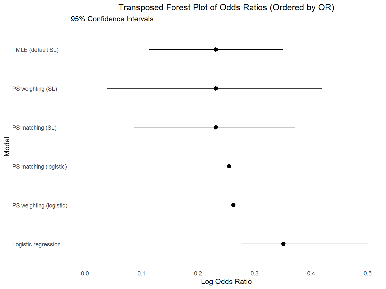
Results comparison

Model	OR	95% CI
Logistic regression	1.42	1.32-1.65
Propensity score matching with logistic	1.29	1.12-1.48
Propensity score weighting with logistic	1.30	1.11-1.53
Propensity score matching with super learner (logistic, LASSO, and XGBoost)	1.26	1.09-1.45
Propensity score weighting with super learner (logistic, LASSO, and XGBoost)	1.26	1.04-1.52
TMLE (default SL library)	1.26	1.12-1.42