
Exercise 1 (W)
Tip
You cannot input any codes on this website but need to download the exercise files on your computer. You can download all of the related files in a zip file wranglingEx.zip from Github folder folder, or just by clicking this link directly.
- Navigate to the GitHub folder (above link) where the ZIP file is located.
- Click on the file name (above zip file) to open its preview window.
- Click on the Download button to download the file. If you can’t see the Download button, click on “Download Raw File” link that should appear on the page.
Important
Once you download and unzip the files, you should see the following files:
- You will work with the file
wranglingE.RMD
Important
Before you start:
You need R and RStudio to complete this exercise. See the R basics chapter on how to download and install R and RStudio on your computer.
Please knit your file at least once and check whether a pdf file is created. See the R Markdown chapter if you need help regarding working with an RMD file.
Problem Statement
Use the functions we learned in Lab 1 to complete Lab 1 Exercise. We will use Right Heart Catheterization Dataset saved in the folder named ‘Data/wrangling/’. The variable list and description can be accessed from Vanderbilt Biostatistics website.
You can access the original table from this paper (doi: 10.1001/jama.1996.03540110043030). We have modified the table and corrected some issues. Please knit your file once you finished and submit the knitted file ONLY.
Problem 1: Basic Manipulation [60%]
- Continuous to Categories: Change the Age variable into categories below 50, 50 to below 60, 60 to below 70, 70 to below 80, 80 and above [Hint: the
cutfunction could be helpful]
- Re-order: Re-order the levels of race to white, black and other
- Set reference: Change the reference category for gender to Male
- Count levels: Check how many levels does the variable “cat1” (Primary disease category) have? Regroup the levels for disease categories to “ARF”,“CHF”,“MOSF”,“Other”. [Hint: the
nlevelsandlistfunctions could be helpful]
- Rename levels: Rename the levels of “ca” (Cancer) to “Metastatic”,“None” and “Localized (Yes)”, then re-order the levels to “None”,“Localized (Yes)” and “Metastatic”
- comorbidities:
- Create a new variable called “numcom” to count number of comorbidities illness for each person (12 categories) [Hint: the
rowSumscommand could be helpful], - Report maximum and minimum values of numcom:
- Anlaytic data: Create a dataset that has only the following variables
age, sex, race, cat1, ca, dnr1, aps1, surv2md1, numcom, adld3p, das2d3pc, temp1, hrt1, meanbp1, resp1, wblc1, pafi1, paco21, ph1, crea1, alb1, scoma1, swang1
name the dataset as rhc2
Problem 2: Table 1 [10%]
Re-produce the sample table 1 from the rhc2 data (see the Table below). In your table, the variables should be ordered as the same as the sample. Please re-level or re-order the levels if needed. [Hint: the tableone package might be useful]
| No RHC | RHC | |
|---|---|---|
| n | 3551 | 2184 |
| age (%) | ||
| [-Inf,50) | 884 (24.9) | 540 (24.7) |
| [50,60) | 546 (15.4) | 371 (17.0) |
| [60,70) | 812 (22.9) | 577 (26.4) |
| [70,80) | 809 (22.8) | 529 (24.2) |
| [80, Inf) | 500 (14.1) | 167 ( 7.6) |
| sex = Female (%) | 1637 (46.1) | 906 (41.5) |
| race (%) | ||
| white | 2753 (77.5) | 1707 (78.2) |
| black | 585 (16.5) | 335 (15.3) |
| other | 213 ( 6.0) | 142 ( 6.5) |
| cat1 (%) | ||
| ARF | 1581 (44.5) | 909 (41.6) |
| CHF | 247 ( 7.0) | 209 ( 9.6) |
| Other | 955 (26.9) | 208 ( 9.5) |
| MOSF | 768 (21.6) | 858 (39.3) |
| ca (%) | ||
| None | 2652 (74.7) | 1727 (79.1) |
| Localized (Yes) | 638 (18.0) | 334 (15.3) |
| Metastatic | 261 ( 7.4) | 123 ( 5.6) |
| dnr1 = Yes (%) | 499 (14.1) | 155 ( 7.1) |
| aps1 (mean (SD)) | 50.93 (18.81) | 60.74 (20.27) |
| surv2md1 (mean (SD)) | 0.61 (0.19) | 0.57 (0.20) |
| numcom (mean (SD)) | 1.52 (1.17) | 1.48 (1.13) |
| adld3p (mean (SD)) | 1.24 (1.86) | 1.02 (1.69) |
| das2d3pc (mean (SD)) | 20.37 (5.48) | 20.70 (5.03) |
| temp1 (mean (SD)) | 37.63 (1.74) | 37.59 (1.83) |
| hrt1 (mean (SD)) | 112.87 (40.94) | 118.93 (41.47) |
| meanbp1 (mean (SD)) | 84.87 (38.87) | 68.20 (34.24) |
| resp1 (mean (SD)) | 28.98 (13.95) | 26.65 (14.17) |
| wblc1 (mean (SD)) | 15.26 (11.41) | 16.27 (12.55) |
| pafi1 (mean (SD)) | 240.63 (116.66) | 192.43 (105.54) |
| paco21 (mean (SD)) | 39.95 (14.24) | 36.79 (10.97) |
| ph1 (mean (SD)) | 7.39 (0.11) | 7.38 (0.11) |
| crea1 (mean (SD)) | 1.92 (2.03) | 2.47 (2.05) |
| alb1 (mean (SD)) | 3.16 (0.67) | 2.98 (0.93) |
| scoma1 (mean (SD)) | 22.25 (31.37) | 18.97 (28.26) |
Problem 3: Table 1 for subset [10%]
Produce a similar table as Problem 2 but with only male sex and ARF primary disease category (cat1). Add the overall column in the same table. [Hint: filter command could be useful]
Problem 4: Considering eligibility criteria [20%]
Produce a similar table as Problem 2 but only for the subjects who meet all of the following eligibility criteria: (i) age is equal to or above 50, (ii) age is below 80 (iii) Glasgow Coma Score is below 61 and (iv) Primary disease categories are either ARF or MOSF. [Hint: droplevels.data.frame can be a useful function]
Optional [0%]
Optional 1: Missing values
- Any variables included in rhc2 data had missing values? Name that variable. [Hint:
applyfunction could be helpful]
- Count how many NAs does that variable have?
- Produce a table 1 for a complete case data (no missing observations) stratified by
swang1.
Optional 2: Calculating variance of a sample
Write a function for Bessel’s correction to calculate an unbiased estimate of the population variance from a finite sample (a vector of 100 observations, consisting of numbers from 1 to 100).
Hint: Take a closer look at the functions, loops and algorithms shown in lab materials. Use a for loop, utilizing the following pseudocode of the algorithm:
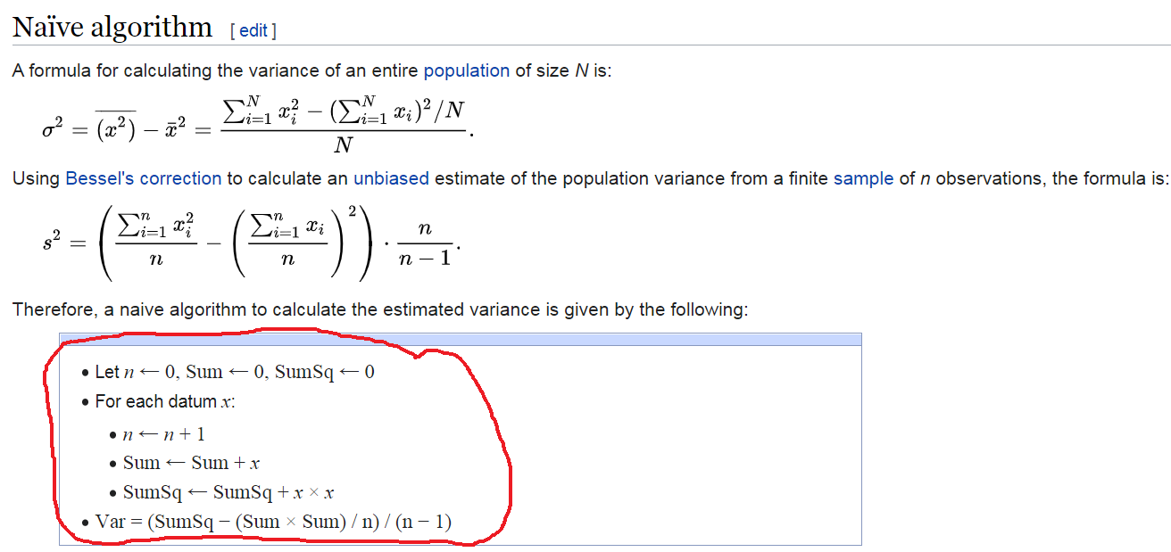
Verify that estimated variance with the following variance function output in R: