Predictive question-2b

Working with a Predictive question using NHANES

Part 2: Analysis of downloaded data:

This tutorial provides a comprehensive guide to NHANES data preparation and initial analysis using R. The tutorial covers topics such as loading dataset, variable recoding, data summary statistics, and various types of regression analyses, including bivariate and multivariate models. It also delves into dealing with missing data, first by omitting NA values for a complete case analysis and then using a simple imputation method. The guide is designed to walk the reader through each step of data manipulation and analysis, with a focus on avoiding common pitfalls in statistical analysis.

Example article

We are continuing to use the article by Li et al. (2020) as our reference. DOI:10.1038/s41371-019-0224-9.

(Li et al. 2020)

Video content (optional)

Tip

For those who prefer a video walkthrough, feel free to watch the video below, which offers a description of an earlier version of the content.

Loading saved data

The following code chunk loads an RData file named that was saved in the previous step. The RData file typically contains saved R objects like data frames, lists, etc.

load("Data/researchquestion/Analytic2013.RData")

The following code lists all the objects in the current workspace.

ls()
#> [1] "analytic.data"   "has_annotations"

The following shows the column names of the analytic.data data frame.

names(analytic.data)
#>  [1] "SEQN"     "RIAGENDR" "RIDAGEYR" "RIDRETH3" "DMDMARTL" "WTINT2YR"
#>  [7] "WTMEC2YR" "SDMVPSU"  "SDMVSTRA" "BPXDI1"   "BPXSY1"   "SMQ040"  
#> [13] "ALQ130"

The following provides summary statistics for the column BPXDI1 in the analytic.data data frame.

summary(analytic.data$BPXDI1)
#>    Min. 1st Qu.  Median    Mean 3rd Qu.    Max.    NA's 
#>    0.00   58.00   66.00   65.77   76.00  122.00    3003

Target

First, we need to understand the data well. What is the common support in all of the population?

Variable	Target
SEQN	Both males and females 0 YEARS - 150 YEARS
RIAGENDR	Both males and females 0 YEARS - 150 YEARS
RIDAGEYR	Both males and females 0 YEARS - 150 YEARS
RIDRETH3	Both males and females 0 YEARS - 150 YEARS
DMDMARTL	Both males and females 20 YEARS - 150 YEARS
WTINT2YR	Both males and females 0 YEARS - 150 YEARS
WTMEC2YR	Both males and females 0 YEARS - 150 YEARS
SDMVPSU	Both males and females 0 YEARS - 150 YEARS
SDMVSTRA	Both males and females 0 YEARS - 150 YEARS
BPXDI1	Both males and females 8 YEARS - 150 YEARS
BPXSY1	Both males and females 8 YEARS - 150 YEARS
SMQ040	Both males and females 18 YEARS - 150 YEARS
ALQ130	Both males and females 18 YEARS - 150 YEARS
-	-

Both males and females 20 YEARS - 150 YEARS. The study should be restricted to age 20 and +.

Recode and Univariate summary

Blood pressure

require(car)
summary(analytic.data$BPXSY1)
#>    Min. 1st Qu.  Median    Mean 3rd Qu.    Max.    NA's 
#>    66.0   106.0   116.0   118.1   128.0   228.0    3003
summary(analytic.data$BPXDI1)
#>    Min. 1st Qu.  Median    Mean 3rd Qu.    Max.    NA's 
#>    0.00   58.00   66.00   65.77   76.00  122.00    3003
# what is 0 blood pressure?
# change all 0 to NA
analytic.data$BPXDI1 <- recode(analytic.data$BPXDI1, "0=NA") 

#create a new variable
analytic.data$blood.pressure <- analytic.data$BPXDI1 

# delete old variable
analytic.data$BPXDI1 <- NULL

# check summary
summary(analytic.data$blood.pressure)
#>    Min. 1st Qu.  Median    Mean 3rd Qu.    Max.    NA's 
#>    4.00   58.00   68.00   66.54   76.00  122.00    3086

Race

The RIDRETH3 column is recoded to simplify racial categories.

analytic.data$RIDRETH3 <- 
  recode(analytic.data$RIDRETH3,
         "c('Non-Hispanic Asian',
         'Other Race - Including Multi-Rac')='Other race'")
analytic.data$race <- analytic.data$RIDRETH3
analytic.data$RIDRETH3 <- NULL
table(analytic.data$race,useNA="always")
#> 
#>   Mexican American Non-Hispanic Black Non-Hispanic White     Other Hispanic 
#>               1730               2267               3674                960 
#>         Other race               <NA> 
#>               1544                  0

Age (centering)

Age values are centered around the mean age for those who are 20 years or older.

summary(analytic.data$RIDAGEYR)
#>    Min. 1st Qu.  Median    Mean 3rd Qu.    Max. 
#>    0.00   10.00   26.00   31.48   52.00   80.00
centre.adult <- mean(analytic.data$RIDAGEYR[analytic.data$RIDAGEYR 
                                            >= 20], na.rm = TRUE)
centre.adult
#> [1] 49.11111
# This is actually not the correct mean age. Guess why?
# Hint: see the NHANES data dictionary for age variable.
analytic.data$RIDAGEYRc <- analytic.data$RIDAGEYR - centre.adult
analytic.data$age.centred <- analytic.data$RIDAGEYRc
analytic.data$RIDAGEYRc <- NULL
summary(analytic.data$age.centred)
#>    Min. 1st Qu.  Median    Mean 3rd Qu.    Max. 
#> -49.111 -39.111 -23.111 -17.627   2.889  30.889

Gender

A new column gender is created for gender details.

analytic.data$gender <- analytic.data$RIAGENDR
analytic.data$RIAGENDR <- NULL
table(analytic.data$gender, useNA = "always")
#> 
#>   Male Female   <NA> 
#>   5003   5172      0

Marital status

The marital status is simplified.

summary(analytic.data$DMDMARTL)
#>             Married             Widowed            Divorced           Separated 
#>                2965                 436                 659                 177 
#>       Never married Living with partner             Refused          Don't Know 
#>                1112                 417                   2                   1 
#>                NA's 
#>                4406
analytic.data$DMDMARTL <- 
  recode(analytic.data$DMDMARTL, 
  "c('Widowed','Divorced','Separated')='Previously married';
  c('Living with partner','Married')='Married'; 
  'Never married' = 'Never married';
  else=NA")

# what happened to 77 and 99? Hint: else
analytic.data$marital <- analytic.data$DMDMARTL 
analytic.data$DMDMARTL <- NULL
table(analytic.data$marital, useNA = "always")
#> 
#>            Married      Never married Previously married               <NA> 
#>               3382               1112               1272               4409

Alcohol

For Alcohol, codes like 777 and 999 are converted to NA.

summary(analytic.data$ALQ130)
#>    Min. 1st Qu.  Median    Mean 3rd Qu.    Max.    NA's 
#>   1.000   1.000   2.000   3.511   3.000 999.000    6579
# what is  777 and 999? See NHANES data dictionary.
# Refused and Don't know
analytic.data$ALQ130[analytic.data$ALQ130 == 999] <- NA
analytic.data$ALQ130[analytic.data$ALQ130 == 777] <- NA
analytic.data$alcohol <- analytic.data$ALQ130
analytic.data$ALQ130 <- NULL
table(analytic.data$alcohol, useNA = "always")
#> 
#>    1    2    3    4    5    6    7    8    9   10   11   12   13   14   15   16 
#> 1280 1002  536  283  154  156   23   54    4   28    4   43    5    2    6    4 
#>   18   20   24   25 <NA> 
#>    3    4    1    1 6582

Smoking

Similar to alcohol, unusual codes are converted to NA.

summary(analytic.data$SMQ040)
#>  Every day  Some days Not at all       NA's 
#>        992        240       1347       7596
# what is  7 and 9? See NHANES data dictionary.
# Refused and Don't know
analytic.data$SMQ040[analytic.data$SMQ040 == 9] <- NA
analytic.data$SMQ040[analytic.data$SMQ040 == 7] <- NA
analytic.data$smoke <- analytic.data$SMQ040
analytic.data$SMQ040 <- NULL
table(analytic.data$smoke, useNA = "always")
#> 
#>  Every day  Some days Not at all       <NA> 
#>        992        240       1347       7596

Renaming

Columns in the data frame are renamed for better readability.

names(analytic.data)
#>  [1] "SEQN"           "RIDAGEYR"       "WTINT2YR"       "WTMEC2YR"      
#>  [5] "SDMVPSU"        "SDMVSTRA"       "BPXSY1"         "blood.pressure"
#>  [9] "race"           "age.centred"    "gender"         "marital"       
#> [13] "alcohol"        "smoke"

Order is important.

names(analytic.data) <- c("id", "age", "w.all", "w.MEC", 
                          "PSU", "STRATA", "systolic", 
                          "diastolic", "race", "age.centred", 
                          "gender", "marital", "alcohol", 
                          "smoke")

names(analytic.data)
#>  [1] "id"          "age"         "w.all"       "w.MEC"       "PSU"        
#>  [6] "STRATA"      "systolic"    "diastolic"   "race"        "age.centred"
#> [11] "gender"      "marital"     "alcohol"     "smoke"

Subsetting to avoid zero-cells

A new age category (age.cat) is created to segregate the data. Remember that, the target for marital status component was 20 YEARS - 150 YEARS.

summary(analytic.data$age)
#>    Min. 1st Qu.  Median    Mean 3rd Qu.    Max. 
#>    0.00   10.00   26.00   31.48   52.00   80.00

analytic.data$age.cat <- cut(analytic.data$age, 
                             breaks = c(-Inf, 20,50,+Inf), 
                             right = FALSE)

table(analytic.data$age.cat)
#> 
#> [-Inf,20)   [20,50) [50, Inf) 
#>      4406      2989      2780

summary(analytic.data$alcohol)
#>    Min. 1st Qu.  Median    Mean 3rd Qu.    Max.    NA's 
#>    1.00    1.00    2.00    2.68    3.00   25.00    6582

table(analytic.data$age.cat, analytic.data$marital)
#>            
#>             Married Never married Previously married
#>   [-Inf,20)       0             0                  0
#>   [20,50)      1771           890                327
#>   [50, Inf)    1611           222                945

dim(analytic.data)
#> [1] 10175    15
analytic.data1 <- subset(analytic.data , 
                         !is.na(age) & age >= 20)
dim(analytic.data1)
#> [1] 5769   15

Note: This subsetting is problematic for further survey data analysis. We will learn to work with this subsetting correctly later.

analytic.data1$age <-NULL

Summary

This part provides various summary statistics for the processed data.

Univariate summary for the complete case

summary(analytic.data1$diastolic)
#>    Min. 1st Qu.  Median    Mean 3rd Qu.    Max.    NA's 
#>     4.0    62.0    70.0    70.3    78.0   122.0     686

table(analytic.data1$race,useNA = "always")
#> 
#>   Mexican American Non-Hispanic Black Non-Hispanic White     Other Hispanic 
#>                767               1177               2472                508 
#>         Other race               <NA> 
#>                845                  0

summary(analytic.data1$age.centred)
#>    Min. 1st Qu.  Median    Mean 3rd Qu.    Max. 
#> -29.111 -15.111  -1.111   0.000  13.889  30.889

table(analytic.data1$gender,useNA = "always")
#> 
#>   Male Female   <NA> 
#>   2758   3011      0

table(analytic.data1$marital,useNA = "always")
#> 
#>            Married      Never married Previously married               <NA> 
#>               3382               1112               1272                  3

Saving for further use

save(analytic.data1, 
     file = "Data/researchquestion/NHANESanalytic.Rdata")

Regression summary (Optional)

This is optional content for this chapter. Later in confounding and predictive factor chapters, we will learn more about adjustment.

Different Generalized Linear Models (GLMs) are fit for diastolic blood pressure using variables like gender, marital status, etc. Below, we used GLMs with the Gaussian family for the continuous outcome diastolic. Note that gaussian is the default family for the glm function. Some other family options include binomial, poisson, quasibinomial, and so on.

Bivariate Regression summary (missing values included)

fit1g <- glm(diastolic ~ gender, data = analytic.data1)
summary(fit1g)
#> 
#> Call:
#> glm(formula = diastolic ~ gender, data = analytic.data1)
#> 
#> Deviance Residuals: 
#>     Min       1Q   Median       3Q      Max  
#> -67.579   -7.091    0.421    6.909   50.421  
#> 
#> Coefficients:
#>              Estimate Std. Error t value Pr(>|t|)    
#> (Intercept)   71.5789     0.2352 304.299  < 2e-16 ***
#> genderFemale  -2.4880     0.3278  -7.591 3.76e-14 ***
#> ---
#> Signif. codes:  0 '***' 0.001 '**' 0.01 '*' 0.05 '.' 0.1 ' ' 1
#> 
#> (Dispersion parameter for gaussian family taken to be 136.3911)
#> 
#>     Null deviance: 700862  on 5082  degrees of freedom
#> Residual deviance: 693003  on 5081  degrees of freedom
#>   (686 observations deleted due to missingness)
#> AIC: 39415
#> 
#> Number of Fisher Scoring iterations: 2

fit1m <- glm(diastolic ~ marital, data=analytic.data1)
summary(fit1m)
#> 
#> Call:
#> glm(formula = diastolic ~ marital, data = analytic.data1)
#> 
#> Deviance Residuals: 
#>     Min       1Q   Median       3Q      Max  
#> -66.750   -6.838    1.162    7.250   51.250  
#> 
#> Coefficients:
#>                           Estimate Std. Error t value Pr(>|t|)    
#> (Intercept)                70.7500     0.2138 330.901  < 2e-16 ***
#> maritalNever married       -1.9116     0.4316  -4.429 9.69e-06 ***
#> maritalPreviously married  -0.3953     0.4140  -0.955     0.34    
#> ---
#> Signif. codes:  0 '***' 0.001 '**' 0.01 '*' 0.05 '.' 0.1 ' ' 1
#> 
#> (Dispersion parameter for gaussian family taken to be 137.5101)
#> 
#>     Null deviance: 700840  on 5079  degrees of freedom
#> Residual deviance: 698139  on 5077  degrees of freedom
#>   (689 observations deleted due to missingness)
#> AIC: 39434
#> 
#> Number of Fisher Scoring iterations: 2

str(analytic.data1)
#> 'data.frame':    5769 obs. of  14 variables:
#>  $ id         : num  73557 73558 73559 73561 73562 ...
#>  $ w.all      : num  13281 23682 57215 63710 24978 ...
#>  $ w.MEC      : num  13481 24472 57193 65542 25345 ...
#>  $ PSU        : num  1 1 1 2 1 1 2 1 2 2 ...
#>  $ STRATA     : num  112 108 109 116 111 114 106 112 112 113 ...
#>  $ systolic   : num  122 156 140 136 160 118 NA 128 140 106 ...
#>  $ diastolic  : num  72 62 90 86 84 80 NA 74 78 60 ...
#>  $ race       : Factor w/ 5 levels "Mexican American",..: 2 3 3 3 1 3 4 3 3 3 ...
#>  $ age.centred: num  19.89 4.89 22.89 23.89 6.89 ...
#>  $ gender     : Factor w/ 2 levels "Male","Female": 1 1 1 2 1 2 1 2 1 2 ...
#>  $ marital    : Factor w/ 3 levels "Married","Never married",..: 3 1 1 1 3 3 1 3 3 2 ...
#>  $ alcohol    : num  1 4 NA NA 1 1 NA 1 3 2 ...
#>  $ smoke      : Factor w/ 3 levels "Every day","Some days",..: 3 2 3 NA 3 NA 3 1 1 NA ...
#>  $ age.cat    : Factor w/ 3 levels "[-Inf,20)","[20,50)",..: 3 3 3 3 3 3 2 3 3 2 ...
fit13 <- glm(diastolic ~ gender + age.centred + race + 
               marital + systolic + smoke + alcohol, 
             data = analytic.data1)
summary(fit13)
#> 
#> Call:
#> glm(formula = diastolic ~ gender + age.centred + race + marital + 
#>     systolic + smoke + alcohol, data = analytic.data1)
#> 
#> Deviance Residuals: 
#>     Min       1Q   Median       3Q      Max  
#> -75.142   -6.090    0.811    7.074   33.512  
#> 
#> Coefficients:
#>                           Estimate Std. Error t value Pr(>|t|)    
#> (Intercept)               30.92372    2.44895  12.627  < 2e-16 ***
#> genderFemale              -0.34850    0.59830  -0.582 0.560325    
#> age.centred               -0.13638    0.02142  -6.367 2.56e-10 ***
#> raceNon-Hispanic Black     1.44736    1.11246   1.301 0.193443    
#> raceNon-Hispanic White     0.59565    0.96117   0.620 0.535540    
#> raceOther Hispanic         1.07369    1.29793   0.827 0.408234    
#> raceOther race             2.02908    1.22998   1.650 0.099216 .  
#> maritalNever married      -2.92801    0.79123  -3.701 0.000223 ***
#> maritalPreviously married  0.44754    0.71911   0.622 0.533804    
#> systolic                   0.31071    0.01763  17.624  < 2e-16 ***
#> smokeSome days            -0.42177    0.97853  -0.431 0.666513    
#> smokeNot at all            0.01796    0.65159   0.028 0.978008    
#> alcohol                    0.17287    0.10994   1.572 0.116060    
#> ---
#> Signif. codes:  0 '***' 0.001 '**' 0.01 '*' 0.05 '.' 0.1 ' ' 1
#> 
#> (Dispersion parameter for gaussian family taken to be 117.7142)
#> 
#>     Null deviance: 219477  on 1515  degrees of freedom
#> Residual deviance: 176924  on 1503  degrees of freedom
#>   (4253 observations deleted due to missingness)
#> AIC: 11546
#> 
#> Number of Fisher Scoring iterations: 2

Check missingness (optional)

A subsequent chapter will delve into the additional factors that impact how we handle missing data.

The plot_missing() function from the DataExplorer package is used to plot missing data.

require(DataExplorer)
plot_missing(analytic.data1)

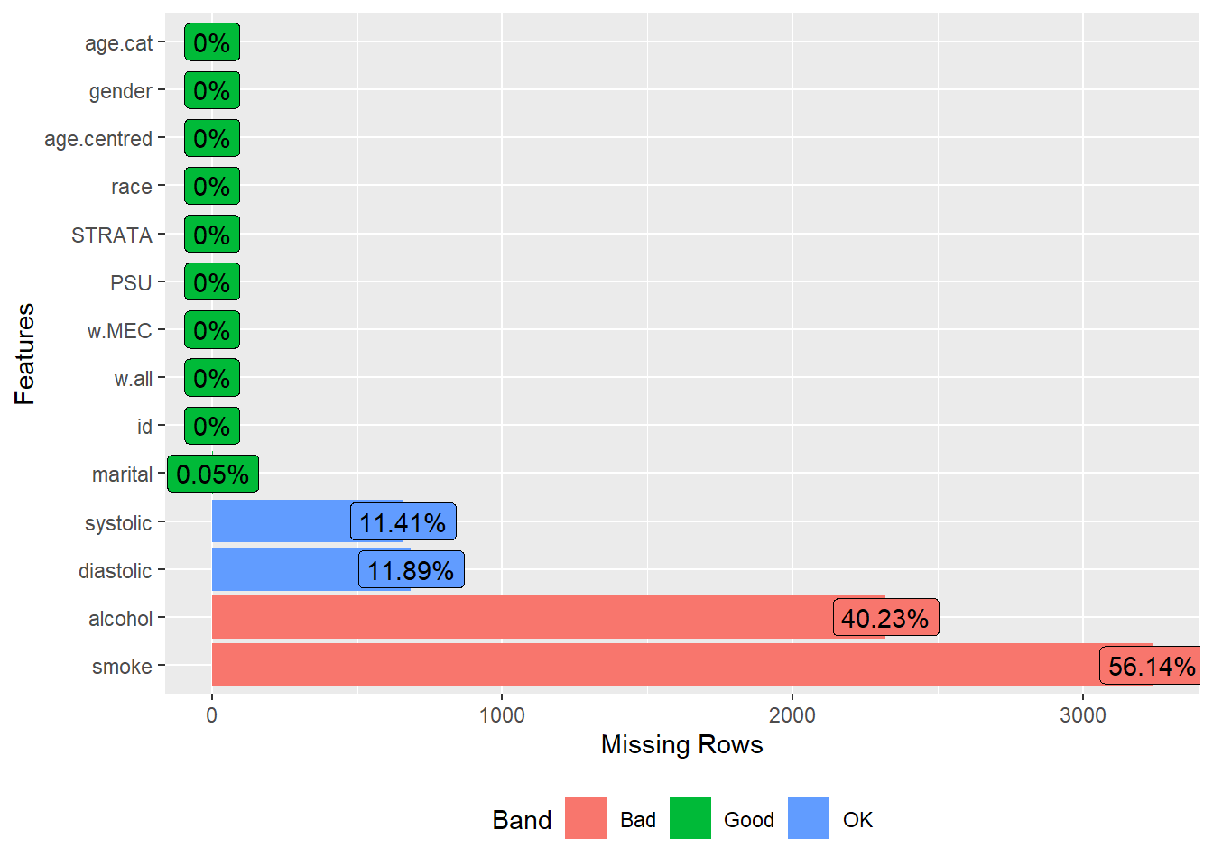
require("tableone")
vars = c("systolic", "smoke", "diastolic", "race", 
         "age.centred", "gender", "marital", "alcohol")
CreateTableOne(data = analytic.data1, includeNA = TRUE, 
               vars = vars)
#>                          
#>                           Overall       
#>   n                         5769        
#>   systolic (mean (SD))    123.16 (18.12)
#>   smoke (%)                             
#>      Every day               965 (16.7) 
#>      Some days               229 ( 4.0) 
#>      Not at all             1336 (23.2) 
#>      NA                     3239 (56.1) 
#>   diastolic (mean (SD))    70.30 (11.74)
#>   race (%)                              
#>      Mexican American        767 (13.3) 
#>      Non-Hispanic Black     1177 (20.4) 
#>      Non-Hispanic White     2472 (42.8) 
#>      Other Hispanic          508 ( 8.8) 
#>      Other race              845 (14.6) 
#>   age.centred (mean (SD))   0.00 (17.56)
#>   gender = Female (%)       3011 (52.2) 
#>   marital (%)                           
#>      Married                3382 (58.6) 
#>      Never married          1112 (19.3) 
#>      Previously married     1272 (22.0) 
#>      NA                        3 ( 0.1) 
#>   alcohol (mean (SD))       2.65 (2.34)

Setting correct variable types

The variables are explicitly set to either numeric or factor types.

Note: In case any of the variables types are wrong, your table 1 output will be wrong. Better to be sure about what type of variable you want them to be (numeric or factor). For example, systolic should be numeric. Is it defined that way?

mode(analytic.data1$systolic)
#> [1] "numeric"

In case it wasn’t (often they can get converted to character), then here is the solution:

# solution 1: one-by-one
analytic.data1$systolic <- 
  as.numeric(as.character(analytic.data1$systolic))
summary(analytic.data1$systolic)
#>    Min. 1st Qu.  Median    Mean 3rd Qu.    Max.    NA's 
#>    66.0   110.0   120.0   123.2   134.0   228.0     658

# solution 2: fixing all variable types at once
numeric.names <- c("systolic", "diastolic", 
                   "age.centred", "alcohol")
factor.names <- vars[!vars %in% numeric.names]
factor.names
#> [1] "smoke"   "race"    "gender"  "marital"
analytic.data1[,factor.names] <- 
  lapply(analytic.data1[,factor.names] , factor)
analytic.data1[numeric.names] <- 
  apply(X = analytic.data1[numeric.names], MARGIN = 2, 
        FUN =function (x) as.numeric(as.character(x)))
levels(analytic.data1$marital)
#> [1] "Married"            "Never married"      "Previously married"
CreateTableOne(data = analytic.data1, includeNA = TRUE, 
               vars = vars)
#>                          
#>                           Overall       
#>   n                         5769        
#>   systolic (mean (SD))    123.16 (18.12)
#>   smoke (%)                             
#>      Every day               965 (16.7) 
#>      Some days               229 ( 4.0) 
#>      Not at all             1336 (23.2) 
#>      NA                     3239 (56.1) 
#>   diastolic (mean (SD))    70.30 (11.74)
#>   race (%)                              
#>      Mexican American        767 (13.3) 
#>      Non-Hispanic Black     1177 (20.4) 
#>      Non-Hispanic White     2472 (42.8) 
#>      Other Hispanic          508 ( 8.8) 
#>      Other race              845 (14.6) 
#>   age.centred (mean (SD))   0.00 (17.56)
#>   gender = Female (%)       3011 (52.2) 
#>   marital (%)                           
#>      Married                3382 (58.6) 
#>      Never married          1112 (19.3) 
#>      Previously married     1272 (22.0) 
#>      NA                        3 ( 0.1) 
#>   alcohol (mean (SD))       2.65 (2.34)

Complete case analysis

Removes all rows containing NA.

dim(analytic.data1)
#> [1] 5769   14
analytic.data2 <- as.data.frame(na.omit(analytic.data1))
dim(analytic.data2)
#> [1] 1516   14
plot_missing(analytic.data2)

tab1 <- CreateTableOne(data = analytic.data2, includeNA = TRUE, 
               vars = vars)
print(tab1)
#>                          
#>                           Overall       
#>   n                         1516        
#>   systolic (mean (SD))    123.29 (17.58)
#>   smoke (%)                             
#>      Every day               590 (38.9) 
#>      Some days               159 (10.5) 
#>      Not at all              767 (50.6) 
#>   diastolic (mean (SD))    70.11 (12.04)
#>   race (%)                              
#>      Mexican American        162 (10.7) 
#>      Non-Hispanic Black      292 (19.3) 
#>      Non-Hispanic White      778 (51.3) 
#>      Other Hispanic          126 ( 8.3) 
#>      Other race              158 (10.4) 
#>   age.centred (mean (SD))  -0.76 (16.71)
#>   gender = Female (%)        626 (41.3) 
#>   marital (%)                           
#>      Married                 858 (56.6) 
#>      Never married           300 (19.8) 
#>      Previously married      358 (23.6) 
#>   alcohol (mean (SD))       3.15 (2.76)
# For categorical variables, try to see if 
# any categories have 0% or 100% frequency.
# If yes, those may create problem in further analysis.

We can export the tableone to a csv file as follows:

tabl1p <- print(tab1)
#>                          
#>                           Overall       
#>   n                         1516        
#>   systolic (mean (SD))    123.29 (17.58)
#>   smoke (%)                             
#>      Every day               590 (38.9) 
#>      Some days               159 (10.5) 
#>      Not at all              767 (50.6) 
#>   diastolic (mean (SD))    70.11 (12.04)
#>   race (%)                              
#>      Mexican American        162 (10.7) 
#>      Non-Hispanic Black      292 (19.3) 
#>      Non-Hispanic White      778 (51.3) 
#>      Other Hispanic          126 ( 8.3) 
#>      Other race              158 (10.4) 
#>   age.centred (mean (SD))  -0.76 (16.71)
#>   gender = Female (%)        626 (41.3) 
#>   marital (%)                           
#>      Married                 858 (56.6) 
#>      Never married           300 (19.8) 
#>      Previously married      358 (23.6) 
#>   alcohol (mean (SD))       3.15 (2.76)
write.csv(tabl1p, file = "Data/researchquestion/table1.csv")

fit23 <- glm(diastolic ~ gender + age.centred + race + 
               marital + systolic + smoke + alcohol, 
             data = analytic.data2)
require(Publish)
publish(fit23)
#>     Variable              Units Coefficient         CI.95     p-value 
#>  (Intercept)                          30.92 [26.12;35.72]     < 1e-04 
#>       gender               Male         Ref                           
#>                          Female       -0.35  [-1.52;0.82]   0.5603254 
#>  age.centred                          -0.14 [-0.18;-0.09]     < 1e-04 
#>         race   Mexican American         Ref                           
#>              Non-Hispanic Black        1.45  [-0.73;3.63]   0.1934428 
#>              Non-Hispanic White        0.60  [-1.29;2.48]   0.5355396 
#>                  Other Hispanic        1.07  [-1.47;3.62]   0.4082336 
#>                      Other race        2.03  [-0.38;4.44]   0.0992165 
#>      marital            Married         Ref                           
#>                   Never married       -2.93 [-4.48;-1.38]   0.0002229 
#>              Previously married        0.45  [-0.96;1.86]   0.5338035 
#>     systolic                           0.31   [0.28;0.35]     < 1e-04 
#>        smoke          Every day         Ref                           
#>                       Some days       -0.42  [-2.34;1.50]   0.6665127 
#>                      Not at all        0.02  [-1.26;1.30]   0.9780080 
#>      alcohol                           0.17  [-0.04;0.39]   0.1160603

Imputed data

We will learn about proper missing data analysis at a latter class. Currently, we will do a simple (but rather controversial) single imputation. In here we are simply using a random sampling to impute (probably the worst method, but we are just filling in some gaps for now).

require(mice)
imputation1 <- mice(analytic.data1,
                   method = "sample",  
                   m = 1, # Number of multiple imputations
                   maxit = 1 # #iteration; mostly useful for convergence
                   )
#> 
#>  iter imp variable
#>   1   1  systolic  diastolic  marital  alcohol  smoke
#> Warning: Number of logged events: 5
analytic.data.imputation1 <- complete(imputation1)
dim(analytic.data.imputation1)
#> [1] 5769   14
str(analytic.data.imputation1)
#> 'data.frame':    5769 obs. of  14 variables:
#>  $ id         : num  73557 73558 73559 73561 73562 ...
#>  $ w.all      : num  13281 23682 57215 63710 24978 ...
#>  $ w.MEC      : num  13481 24472 57193 65542 25345 ...
#>  $ PSU        : num  1 1 1 2 1 1 2 1 2 2 ...
#>  $ STRATA     : num  112 108 109 116 111 114 106 112 112 113 ...
#>  $ systolic   : num  122 156 140 136 160 118 180 128 140 106 ...
#>  $ diastolic  : num  72 62 90 86 84 80 84 74 78 60 ...
#>  $ race       : Factor w/ 5 levels "Mexican American",..: 2 3 3 3 1 3 4 3 3 3 ...
#>  $ age.centred: num  19.89 4.89 22.89 23.89 6.89 ...
#>  $ gender     : Factor w/ 2 levels "Male","Female": 1 1 1 2 1 2 1 2 1 2 ...
#>  $ marital    : Factor w/ 3 levels "Married","Never married",..: 3 1 1 1 3 3 1 3 3 2 ...
#>  $ alcohol    : num  1 4 2 1 1 1 2 1 3 2 ...
#>  $ smoke      : Factor w/ 3 levels "Every day","Some days",..: 3 2 3 3 3 3 3 1 1 1 ...
#>  $ age.cat    : Factor w/ 3 levels "[-Inf,20)","[20,50)",..: 3 3 3 3 3 3 2 3 3 2 ...
plot_missing(analytic.data.imputation1)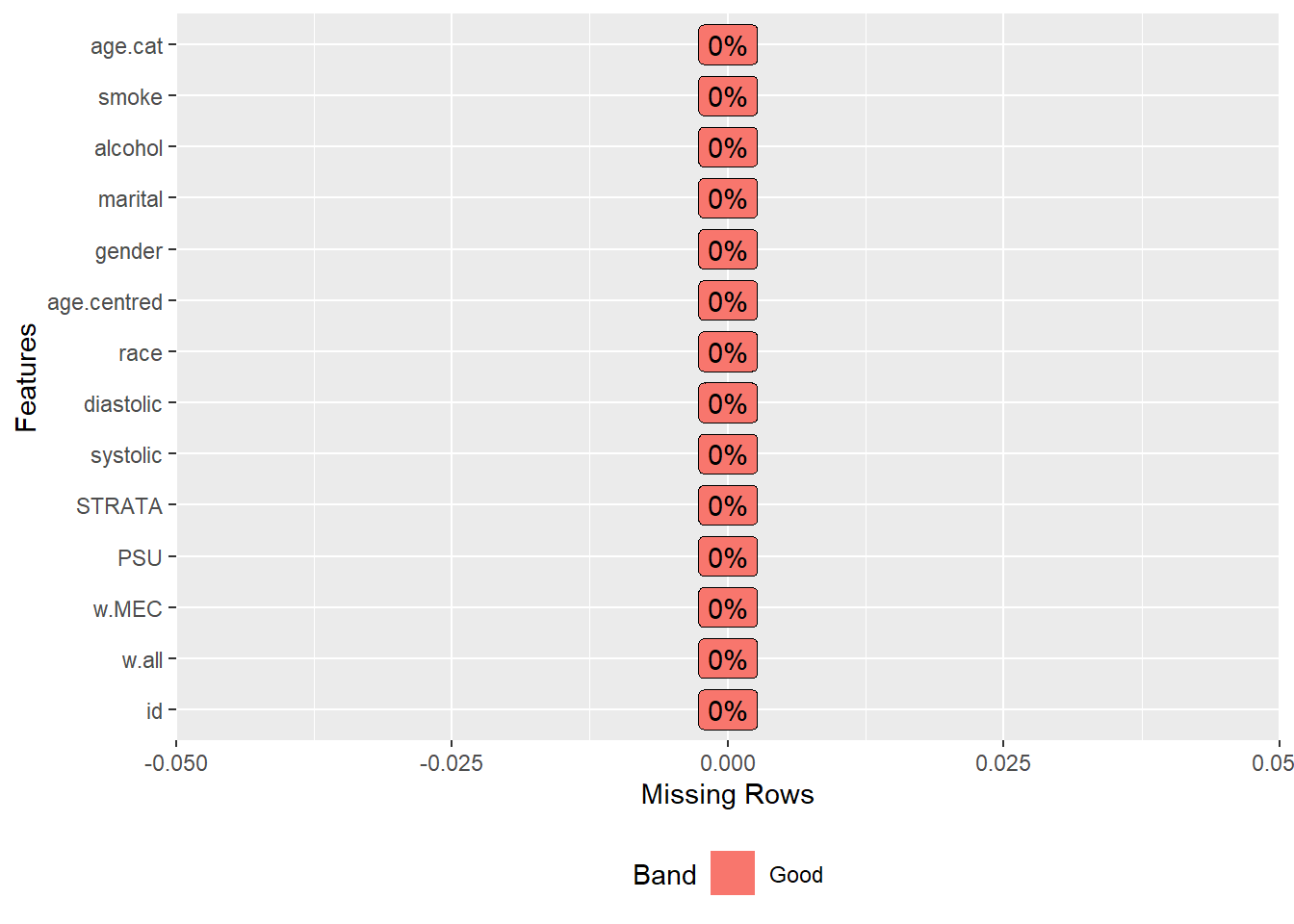

CreateTableOne(data = analytic.data.imputation1, includeNA = TRUE,
               vars = vars)
#>                          
#>                           Overall       
#>   n                         5769        
#>   systolic (mean (SD))    123.17 (18.14)
#>   smoke (%)                             
#>      Every day              2196 (38.1) 
#>      Some days               531 ( 9.2) 
#>      Not at all             3042 (52.7) 
#>   diastolic (mean (SD))    70.33 (11.76)
#>   race (%)                              
#>      Mexican American        767 (13.3) 
#>      Non-Hispanic Black     1177 (20.4) 
#>      Non-Hispanic White     2472 (42.8) 
#>      Other Hispanic          508 ( 8.8) 
#>      Other race              845 (14.6) 
#>   age.centred (mean (SD))   0.00 (17.56)
#>   gender = Female (%)       3011 (52.2) 
#>   marital (%)                           
#>      Married                3384 (58.7) 
#>      Never married          1112 (19.3) 
#>      Previously married     1273 (22.1) 
#>   alcohol (mean (SD))       2.67 (2.36)
# For categorical variables, try to see if 
# any categories have 0% or 100% frequency.
# If yes, those may create problem in further analysis.

fit23i <- glm(diastolic ~ gender + age.centred + race + 
                marital + systolic + smoke + alcohol, 
              data = analytic.data.imputation1)
publish(fit23i)
#>     Variable              Units Coefficient         CI.95    p-value 
#>  (Intercept)                          39.78 [37.44;42.13]    < 1e-04 
#>       gender               Male         Ref                          
#>                          Female       -1.41 [-1.99;-0.83]    < 1e-04 
#>  age.centred                          -0.11 [-0.13;-0.09]    < 1e-04 
#>         race   Mexican American         Ref                          
#>              Non-Hispanic Black        0.75  [-0.26;1.76]   0.146424 
#>              Non-Hispanic White        0.50  [-0.39;1.39]   0.271641 
#>                  Other Hispanic        0.51  [-0.71;1.73]   0.413715 
#>                      Other race        1.43   [0.36;2.50]   0.008652 
#>      marital            Married         Ref                          
#>                   Never married       -2.73 [-3.53;-1.92]    < 1e-04 
#>              Previously married       -0.31  [-1.05;0.43]   0.410962 
#>     systolic                           0.25   [0.24;0.27]    < 1e-04 
#>        smoke          Every day         Ref                          
#>                       Some days       -0.32  [-1.35;0.72]   0.550088 
#>                      Not at all       -0.32  [-0.93;0.28]   0.297969 
#>      alcohol                           0.10  [-0.02;0.22]   0.101564

We see some changes in the estimates. After imputing compared to complete case analysis, any changes dramatic (e.g., changing conclusion)?

Additional factors come into play when dealing with complex survey datasets; these will be explored in a subsequent chapter.

require(jtools)
require(ggstance)
require(broom.mixed)
require(huxtable)
export_summs(fit23, fit23i)

	Model 1	Model 2
(Intercept)	30.92 ***	39.78 ***
	(2.45)	(1.20)
genderFemale	-0.35	-1.41 ***
	(0.60)	(0.29)
age.centred	-0.14 ***	-0.11 ***
	(0.02)	(0.01)
raceNon-Hispanic Black	1.45	0.75
	(1.11)	(0.51)
raceNon-Hispanic White	0.60	0.50
	(0.96)	(0.45)
raceOther Hispanic	1.07	0.51
	(1.30)	(0.62)
raceOther race	2.03	1.43 **
	(1.23)	(0.55)
maritalNever married	-2.93 ***	-2.73 ***
	(0.79)	(0.41)
maritalPreviously married	0.45	-0.31
	(0.72)	(0.38)
systolic	0.31 ***	0.25 ***
	(0.02)	(0.01)
smokeSome days	-0.42	-0.32
	(0.98)	(0.53)
smokeNot at all	0.02	-0.32
	(0.65)	(0.31)
alcohol	0.17	0.10
	(0.11)	(0.06)
N	1516	5769
AIC	11545.85	43937.11
BIC	11620.38	44030.35
Pseudo R2	0.19	0.14
*** p < 0.001; ** p < 0.01; * p < 0.05.

plot_summs(fit23, fit23i)

# plot_summs(fit23, fit23i, plot.distributions = TRUE)

Exercise (try yourself)

In this lab, we have done multiple steps that could be improved. One of them was single imputation by random sampling. What other ad hoc method you could use to impute the factor variables?

References

Li, Meng, Shoumeng Yan, Xing Li, Shan Jiang, Xiaoyu Ma, Hantong Zhao, Jiagen Li, et al. 2020. “Association Between Blood Pressure and Dietary Intakes of Sodium and Potassium Among US Adults Using Quantile Regression Analysis NHANES 2007–2014.” Journal of Human Hypertension 34 (5): 346–54.