PSW with multiple tx
Problem
In this chapter, we will use propensity score weighting (PSW) for multiple treatment categories. We will use CCHS data that was used in the previous chapter on exact matching with CCHS.
Load data
Let us import the dataset:
-
analytic.miss: Full dataset of 397,173 participants from CCHS cycles 1.1, 2.1, and 3.1 with missing values in some covariates -
analytic2: Analytic dataset of 185,613 participants without missing in the covariates.
Pre-processing
Let us create the full and analytic datasets for only CCHS 3.1.
We will use the analytic dataset (dat.analytic) to run our PSW analysis with the following variables: - Outcome: CVD - Exposure: phyact (3-level physical activity) - Covariates: age, sex, married (marital status), race, edu (education), income, bmi (body mass index), doctor (whether visited to a doctor), stress, smoke, drink (drink alcohol or not), fruit (fruit consumption), bp (blood pressure), diab (diabetes), OA (osteoarthritis), immigrate (immigrant or not)
- Sampling weight: weight
# Is there any character variable?
str(dat.analytic)
#> 'data.frame':    39634 obs. of  22 variables:
#>  $ CVD      : chr  "no event" "no event" "no event" "no event" ...
#>  $ age      : chr  "20-29 years" "65 years and over" "20-29 years" "20-29 years" ...
#>  $ sex      : chr  "Male" "Female" "Male" "Female" ...
#>  $ married  : chr  "not single" "single" "single" "single" ...
#>  $ race     : chr  "White" "White" "White" "White" ...
#>  $ edu      : chr  "2nd grad." "Post-2nd grad." "2nd grad." "Other 2nd grad." ...
#>  $ income   : chr  "$50,000-$79,999" "$29,999 or less" "$29,999 or less" "$50,000-$79,999" ...
#>  $ bmi      : Factor w/ 3 levels "Underweight",..: 3 2 2 2 2 3 2 3 3 2 ...
#>  $ phyact   : chr  "Inactive" "Moderate" "Active" "Moderate" ...
#>  $ doctor   : chr  "Yes" "Yes" "Yes" "No" ...
#>  $ stress   : chr  "Not too stressed" "Not too stressed" "Not too stressed" "Not too stressed" ...
#>  $ smoke    : chr  "Former smoker" "Never smoker" "Never smoker" "Never smoker" ...
#>  $ drink    : chr  "Current drinker" "Former driker" "Never drank" "Current drinker" ...
#>  $ fruit    : Factor w/ 3 levels "0-3 daily serving",..: 2 2 1 1 3 2 2 2 2 3 ...
#>  $ bp       : chr  "No" "No" "No" "No" ...
#>  $ diab     : chr  "No" "No" "No" "No" ...
#>  $ province : chr  "South" "South" "South" "South" ...
#>  $ weight   : num  93.5 111.4 120.4 328.2 810.6 ...
#>  $ cycle    : Factor w/ 3 levels "11","21","31": 3 3 3 3 3 3 3 3 3 3 ...
#>  $ ID       : int  264953 264954 264961 264962 264963 264964 264969 264971 264975 264976 ...
#>  $ OA       : chr  "Control" "OA" "Control" "Control" ...
#>  $ immigrate: chr  "not immigrant" "not immigrant" "not immigrant" "not immigrant" ...

# Make all variables (except for ID and weight) as factor
var.names <- c("CVD", "phyact", "age", "sex", "married", "race", "edu", "income", "bmi", "doctor",
               "stress", "smoke", "drink", "fruit", "bp", "diab", "province", "OA", "immigrate")
dat.full[var.names] <- lapply(dat.full[var.names] , factor)
dat.analytic[var.names] <- lapply(dat.analytic[var.names], factor)

# Outcome - CVD
table(dat.analytic$CVD, useNA = "always")
#>
#>    event no event     <NA>
#>     1931    37703        0
dat.full$CVD <- car::recode(dat.full$CVD, "'no event' = 'No'; 'event' = 'Yes'; else = NA ")
dat.full$CVD <- factor(dat.full$CVD, levels = c("No", "Yes"))

dat.analytic$CVD <- car::recode(dat.analytic$CVD, "'no event' = 'No'; 'event' = 'Yes'; else = NA ")
dat.analytic$CVD <- factor(dat.analytic$CVD, levels = c("No", "Yes"))
table(dat.analytic$CVD, useNA = "always")
#>
#>    No   Yes  <NA>
#> 37703  1931     0

# Exposure - physical activity
table(dat.analytic$phyact, useNA = "always")
#>
#>   Active Inactive Moderate     <NA>
#>    11508    17569    10557        0
dat.full$phyact <- factor(dat.full$phyact, levels = c("Inactive", "Moderate", "Active"))
dat.analytic$phyact <- factor(dat.analytic$phyact, levels = c("Inactive", "Moderate", "Active"))

# Table 1
vars <- c("age", "sex", "married", "race", "edu", "income", "bmi", "doctor", "stress",
          "smoke", "drink", "fruit", "bp", "diab", "OA", "immigrate")
tab1 <- CreateTableOne(vars = vars, strata = "phyact", data = dat.analytic, test = F)
print(tab1, smd = T, showAllLevels = T)
#>                Stratified by phyact
#>                 level             Inactive      Moderate      Active
#>   n                               17569         10557         11508
#>   age (%)       20-29 years        2537 (14.4)   1709 (16.2)   2316 (20.1)
#>                 30-39 years        3526 (20.1)   2265 (21.5)   2276 (19.8)
#>                 40-49 years        3270 (18.6)   1939 (18.4)   2037 (17.7)
#>                 50-59 years        2901 (16.5)   1659 (15.7)   1480 (12.9)
#>                 60-64 years        1130 ( 6.4)    665 ( 6.3)    570 ( 5.0)
#>                 65 years and over  3310 (18.8)   1568 (14.9)   1183 (10.3)
#>                 teen                895 ( 5.1)    752 ( 7.1)   1646 (14.3)
#>   sex (%)       Female             9403 (53.5)   5709 (54.1)   5526 (48.0)
#>                 Male               8166 (46.5)   4848 (45.9)   5982 (52.0)
#>   married (%)   not single         9600 (54.6)   5920 (56.1)   5637 (49.0)
#>                 single             7969 (45.4)   4637 (43.9)   5871 (51.0)
#>   race (%)      Non-white          1757 (10.0)    886 ( 8.4)   1066 ( 9.3)
#>                 White             15812 (90.0)   9671 (91.6)  10442 (90.7)
#>   edu (%)       < 2ndary           3690 (21.0)   1635 (15.5)   2039 (17.7)
#>                 2nd grad.          3246 (18.5)   1749 (16.6)   1845 (16.0)
#>                 Other 2nd grad.    1566 ( 8.9)    969 ( 9.2)   1150 (10.0)
#>                 Post-2nd grad.     9067 (51.6)   6204 (58.8)   6474 (56.3)
#>   income (%)    $29,999 or less    4480 (25.5)   1929 (18.3)   1906 (16.6)
#>                 $30,000-$49,999    4018 (22.9)   2059 (19.5)   2097 (18.2)
#>                 $50,000-$79,999    4512 (25.7)   2974 (28.2)   3095 (26.9)
#>                 $80,000 or more    4559 (25.9)   3595 (34.1)   4410 (38.3)
#>   bmi (%)       Underweight         532 ( 3.0)    243 ( 2.3)    340 ( 3.0)
#>                 healthy weight     7349 (41.8)   5023 (47.6)   6233 (54.2)
#>                 Overweight         9688 (55.1)   5291 (50.1)   4935 (42.9)
#>   doctor (%)    No                 2322 (13.2)   1272 (12.0)   1520 (13.2)
#>                 Yes               15247 (86.8)   9285 (88.0)   9988 (86.8)
#>   stress (%)    Not too stressed  13544 (77.1)   8371 (79.3)   9314 (80.9)
#>                 stressed           4025 (22.9)   2186 (20.7)   2194 (19.1)
#>   smoke (%)     Current smoker     5032 (28.6)   2386 (22.6)   2488 (21.6)
#>                 Former smoker      6900 (39.3)   4562 (43.2)   4672 (40.6)
#>                 Never smoker       5637 (32.1)   3609 (34.2)   4348 (37.8)
#>   drink (%)     Current drinker   13913 (79.2)   9016 (85.4)   9863 (85.7)
#>                 Former driker      2582 (14.7)   1102 (10.4)   1063 ( 9.2)
#>                 Never drank        1074 ( 6.1)    439 ( 4.2)    582 ( 5.1)
#>   fruit (%)     0-3 daily serving  5610 (31.9)   2270 (21.5)   1902 (16.5)
#>                 4-6 daily serving  8827 (50.2)   5445 (51.6)   5481 (47.6)
#>                 6+ daily serving   3132 (17.8)   2842 (26.9)   4125 (35.8)
#>   bp (%)        No                14188 (80.8)   8976 (85.0)  10349 (89.9)
#>                 Yes                3381 (19.2)   1581 (15.0)   1159 (10.1)
#>   diab (%)      No                16393 (93.3)  10114 (95.8)  11165 (97.0)
#>                 Yes                1176 ( 6.7)    443 ( 4.2)    343 ( 3.0)
#>   OA (%)        Control           14864 (84.6)   9310 (88.2)  10565 (91.8)
#>                 OA                 2705 (15.4)   1247 (11.8)    943 ( 8.2)
#>   immigrate (%) not immigrant     16557 (94.2)  10150 (96.1)  11098 (96.4)
#>                 recent             1012 ( 5.8)    407 ( 3.9)    410 ( 3.6)
#>                Stratified by phyact
#>                 SMD
#>   n
#>   age (%)        0.285
#>
#>
#>
#>
#>
#>
#>   sex (%)        0.081
#>
#>   married (%)    0.095
#>
#>   race (%)       0.037
#>
#>   edu (%)        0.119
#>
#>
#>
#>   income (%)     0.213
#>
#>
#>
#>   bmi (%)        0.173
#>
#>
#>   doctor (%)     0.023
#>
#>   stress (%)     0.063
#>
#>   smoke (%)      0.129
#>
#>
#>   drink (%)      0.133
#>
#>
#>   fruit (%)      0.323
#>
#>
#>   bp (%)         0.175
#>
#>   diab (%)       0.116
#>
#>   OA (%)         0.150
#>
#>   immigrate (%)  0.070
#>
PSW for multiple tx
Nominal categories (option 1)
For this part (option 1), we consider physical activity as a nominal variable.
Estimating Propensity score
Let us fit the PS model by considering physical activity as a nominal variable and estimate the propensity scores:
# Formula
ps.formula <- formula(phyact ~ age + sex + married + race + edu + income + bmi +
                        doctor + stress + smoke + drink + fruit + bp + diab +
                        OA + immigrate)

# PS model
library(VGAM)
#> Loading required package: stats4
#> Loading required package: splines
#>
#> Attaching package: 'VGAM'
#> The following object is masked from 'package:survey':
#>
#>     calibrate
ps.fit <- vglm(ps.formula, weights = weight, data = dat.analytic,
               family = multinomial(parallel = FALSE))

# Propensity scores
ps <- data.frame(fitted(ps.fit))
head(ps)
# Summary
apply(ps, 2, summary)
#>           Inactive   Moderate    Active
#> Min.    0.06879258 0.07957314 0.0285961
#> 1st Qu. 0.34233334 0.23371928 0.1867680
#> Median  0.44756388 0.27020295 0.2634537
#> Mean    0.44778510 0.26768926 0.2845256
#> 3rd Qu. 0.55452938 0.30446807 0.3616572
#> Max.    0.89058237 0.39864744 0.7524817
Creating weights
Let us create PS weights. For subject \(i\), PS weight is calculated as
\[w_i = \frac{1}{P(A_i = a|L)}, \] where \(A\) is the exposure with levels \(a\) (Inactive, Moderate, and Active in our case), and \(L\) is the list of covariates.
# IPW
dat.analytic$ipw <- ifelse(dat.analytic$phyact=="Active", 1/ps$Active,
                           ifelse(dat.analytic$phyact=="Moderate", 1/ps$Moderate,
                                  1/ps$Inactive))
with(dat.analytic, by(ipw, phyact, summary))
#> phyact: Inactive
#>    Min. 1st Qu.  Median    Mean 3rd Qu.    Max.
#>   1.123   1.671   1.994   2.233   2.505  14.536
#> ------------------------------------------------------------
#> phyact: Moderate
#>    Min. 1st Qu.  Median    Mean 3rd Qu.    Max.
#>   2.508   3.206   3.576   3.743   4.087  11.695
#> ------------------------------------------------------------
#> phyact: Active
#>    Min. 1st Qu.  Median    Mean 3rd Qu.    Max.
#>   1.329   2.310   3.086   3.534   4.225  25.049
Balance checking
Now, we will check the balance in terms of SMD:
library(survey)
vars <- c("age", "sex", "married", "race", "edu", "income", "bmi", "doctor", "stress",
          "smoke", "drink", "fruit", "bp", "diab", "OA", "immigrate")

# Design
w.design <- svydesign(id = ~1, weights = ~ipw, data = dat.analytic)

# Table 1
tabw <- svyCreateTableOne(vars = vars, strata = "phyact", data = w.design, test = F)
print(tabw, smd = T, showAllLevels = T)
#>                Stratified by phyact
#>                 level             Inactive        Moderate
#>   n                               39231.2         39519.8
#>   age (%)       20-29 years        6477.4 (16.5)   6856.1 (17.3)
#>                 30-39 years        7706.8 (19.6)   8174.8 (20.7)
#>                 40-49 years        7098.2 (18.1)   7163.0 (18.1)
#>                 50-59 years        5922.4 (15.1)   5901.2 (14.9)
#>                 60-64 years        2414.8 ( 6.2)   2265.4 ( 5.7)
#>                 65 years and over  6187.1 (15.8)   5843.8 (14.8)
#>                 teen               3424.6 ( 8.7)   3315.4 ( 8.4)
#>   sex (%)       Female            20188.3 (51.5)  20693.4 (52.4)
#>                 Male              19042.9 (48.5)  18826.3 (47.6)
#>   married (%)   not single        20665.9 (52.7)  20907.0 (52.9)
#>                 single            18565.3 (47.3)  18612.8 (47.1)
#>   race (%)      Non-white          3471.9 ( 8.8)   4095.5 (10.4)
#>                 White             35759.3 (91.2)  35424.2 (89.6)
#>   edu (%)       < 2ndary           7267.3 (18.5)   7288.2 (18.4)
#>                 2nd grad.          6902.6 (17.6)   6901.3 (17.5)
#>                 Other 2nd grad.    3783.0 ( 9.6)   3671.6 ( 9.3)
#>                 Post-2nd grad.    21278.3 (54.2)  21658.7 (54.8)
#>   income (%)    $29,999 or less    8432.3 (21.5)   8425.7 (21.3)
#>                 $30,000-$49,999    8115.6 (20.7)   8109.8 (20.5)
#>                 $50,000-$79,999   10169.1 (25.9)  10602.5 (26.8)
#>                 $80,000 or more   12514.2 (31.9)  12381.9 (31.3)
#>   bmi (%)       Underweight        1092.7 ( 2.8)   1110.6 ( 2.8)
#>                 healthy weight    18191.1 (46.4)  18613.7 (47.1)
#>                 Overweight        19947.4 (50.8)  19795.5 (50.1)
#>   doctor (%)    No                 5073.1 (12.9)   5127.6 (13.0)
#>                 Yes               34158.1 (87.1)  34392.2 (87.0)
#>   stress (%)    Not too stressed  30921.0 (78.8)  31245.6 (79.1)
#>                 stressed           8310.3 (21.2)   8274.2 (20.9)
#>   smoke (%)     Current smoker    10018.8 (25.5)  10121.1 (25.6)
#>                 Former smoker     15860.1 (40.4)  15737.2 (39.8)
#>                 Never smoker      13352.4 (34.0)  13661.5 (34.6)
#>   drink (%)     Current drinker   32257.4 (82.2)  32836.4 (83.1)
#>                 Former driker      4857.5 (12.4)   4621.5 (11.7)
#>                 Never drank        2116.4 ( 5.4)   2061.9 ( 5.2)
#>   fruit (%)     0-3 daily serving  9738.2 (24.8)   9786.2 (24.8)
#>                 4-6 daily serving 19523.6 (49.8)  19803.8 (50.1)
#>                 6+ daily serving   9969.4 (25.4)   9929.8 (25.1)
#>   bp (%)        No                33045.9 (84.2)  33662.1 (85.2)
#>                 Yes                6185.3 (15.8)   5857.7 (14.8)
#>   diab (%)      No                37227.0 (94.9)  37572.5 (95.1)
#>                 Yes                2004.2 ( 5.1)   1947.3 ( 4.9)
#>   OA (%)        Control           34297.7 (87.4)  34835.2 (88.1)
#>                 OA                 4933.5 (12.6)   4684.6 (11.9)
#>   immigrate (%) not immigrant     37503.8 (95.6)  37532.8 (95.0)
#>                 recent             1727.4 ( 4.4)   1987.0 ( 5.0)
#>                Stratified by phyact
#>                 Active          SMD
#>   n             40667.9
#>   age (%)        6467.5 (15.9)   0.046
#>                  8588.7 (21.1)
#>                  7538.2 (18.5)
#>                  6327.6 (15.6)
#>                  2420.1 ( 6.0)
#>                  5989.1 (14.7)
#>                  3336.8 ( 8.2)
#>   sex (%)       21026.2 (51.7)   0.012
#>                 19641.7 (48.3)
#>   married (%)   22651.2 (55.7)   0.040
#>                 18016.8 (44.3)
#>   race (%)       3834.0 ( 9.4)   0.034
#>                 36834.0 (90.6)
#>   edu (%)        7395.4 (18.2)   0.023
#>                  6825.8 (16.8)
#>                  3765.2 ( 9.3)
#>                 22681.6 (55.8)
#>   income (%)     8029.8 (19.7)   0.041
#>                  8544.1 (21.0)
#>                 11407.3 (28.0)
#>                 12686.7 (31.2)
#>   bmi (%)        1241.6 ( 3.1)   0.017
#>                 19120.5 (47.0)
#>                 20305.8 (49.9)
#>   doctor (%)     5272.7 (13.0)   0.001
#>                 35395.3 (87.0)
#>   stress (%)    32100.6 (78.9)   0.004
#>                  8567.4 (21.1)
#>   smoke (%)      9760.6 (24.0)   0.032
#>                 17024.0 (41.9)
#>                 13883.4 (34.1)
#>   drink (%)     33927.5 (83.4)   0.022
#>                  4634.1 (11.4)
#>                  2106.3 ( 5.2)
#>   fruit (%)     10170.0 (25.0)   0.007
#>                 20200.6 (49.7)
#>                 10297.3 (25.3)
#>   bp (%)        34372.4 (84.5)   0.017
#>                  6295.6 (15.5)
#>   diab (%)      38850.3 (95.5)   0.020
#>                  1817.7 ( 4.5)
#>   OA (%)        35666.9 (87.7)   0.015
#>                  5001.1 (12.3)
#>   immigrate (%) 38662.6 (95.1)   0.020
#>                  2005.4 ( 4.9)
All covariates are balanced in terms of SMD (SMD \(\le\) 0.20).
Outcome analysis
Now, we will fit the outcome model. To get the correct estimate of the standard error, we will set up the design with full data and subset the design.
# Create an indicator variable in the full dataset
dat.full$ind <- 0
dat.full$ind[dat.full$ID %in% dat.analytic$ID] <- 1

# New weight = IPW * survey weight
dat.analytic$ATEweight <- with(dat.analytic, ipw * weight)

# New weight variable in the full dataset
dat.full$ATEweight <- 0
dat.full$ATEweight[dat.full$ID %in% dat.analytic$ID] <- dat.analytic$ATEweight

# Survey setup with full data
w.design0 <- svydesign(id = ~1, weights = ~ATEweight, data = dat.full)

# Subset the design for analytic sample
w.design1 <- subset(w.design0, ind == 1)

# Weighted proportion
w.prop <- svyby(formula = ~CVD, by = ~phyact, design = w.design1, FUN = svymean)
w.propOrdinal categories (for comparison)
For comparison, let us consider physical activity as a ordinal variable (option 2).
Define ordinal variable
# Exposure - ordinal physical activity
dat.full$phyact.ord <- factor(dat.full$phyact, levels = c("Inactive", "Moderate", "Active"),
                              ordered = T)
dat.analytic$phyact.ord <- factor(dat.analytic$phyact,
                                  levels = c("Inactive", "Moderate", "Active"), ordered = T)
head(dat.analytic$phyact.ord)
#> [1] Inactive Moderate Active   Moderate Active   Active
#> Levels: Inactive < Moderate < Active
Estimating Propensity score
# Formula
ps.formula2 <- formula(phyact.ord ~ age + sex + married + race + edu + income + bmi +
                        doctor + stress + smoke + drink + fruit + bp + diab +
                        OA + immigrate)

# PS model
library(VGAM)
ps.fit2 <- vglm(ps.formula2, weights = weight, data = dat.analytic, family = propodds)

# Propensity scores
ps2 <- data.frame(fitted(ps.fit2))
head(ps2)
# Summary
apply(ps2, 2, summary)
#>           Inactive   Moderate     Active
#> Min.    0.07517679 0.07505615 0.03456101
#> 1st Qu. 0.34108922 0.25002048 0.18907940
#> Median  0.44711595 0.28026693 0.26446898
#> Mean    0.44780744 0.26682382 0.28536874
#> 3rd Qu. 0.55497781 0.29473347 0.35967960
#> Max.    0.89038285 0.29934482 0.78152250
Creating weights
Let us create PS weights:
# IPW
dat.analytic$ipw2 <- ifelse(dat.analytic$phyact=="Active", 1/ps2$Active,
                           ifelse(dat.analytic$phyact=="Moderate", 1/ps2$Moderate,
                                  1/ps2$Inactive))
with(dat.analytic, by(ipw2, phyact.ord, summary))
#> phyact.ord: Inactive
#>    Min. 1st Qu.  Median    Mean 3rd Qu.    Max.
#>   1.123   1.668   2.001   2.237   2.516  13.302
#> ------------------------------------------------------------
#> phyact.ord: Moderate
#>    Min. 1st Qu.  Median    Mean 3rd Qu.    Max.
#>   3.341   3.382   3.525   3.748   3.875  11.248
#> ------------------------------------------------------------
#> phyact.ord: Active
#>    Min. 1st Qu.  Median    Mean 3rd Qu.    Max.
#>   1.280   2.319   3.073   3.504   4.211  19.768
Balance checking
Now, we will check the balance in terms of SMD:
library(survey)
vars <- c("age", "sex", "married", "race", "edu", "income", "bmi", "doctor", "stress",
          "smoke", "drink", "fruit", "bp", "diab", "OA", "immigrate")

# Design
w.design <- svydesign(id = ~1, weights = ~ipw2, data = dat.analytic)

# Table 1
tabw2 <- svyCreateTableOne(vars = vars, strata = "phyact", data = w.design, test = F)
print(tabw2, smd = T, showAllLevels = T)
#>                Stratified by phyact
#>                 level             Inactive        Moderate
#>   n                               39305.5         39566.3
#>   age (%)       20-29 years        6679.4 (17.0)   6125.6 (15.5)
#>                 30-39 years        7635.7 (19.4)   8357.8 (21.1)
#>                 40-49 years        7085.9 (18.0)   7124.1 (18.0)
#>                 50-59 years        5820.8 (14.8)   6307.9 (15.9)
#>                 60-64 years        2339.1 ( 6.0)   2494.0 ( 6.3)
#>                 65 years and over  6108.9 (15.5)   6264.9 (15.8)
#>                 teen               3635.8 ( 9.3)   2892.0 ( 7.3)
#>   sex (%)       Female            19987.1 (50.9)  21622.5 (54.6)
#>                 Male              19318.4 (49.1)  17943.8 (45.4)
#>   married (%)   not single        20342.7 (51.8)  22151.4 (56.0)
#>                 single            18962.9 (48.2)  17414.9 (44.0)
#>   race (%)      Non-white          3595.2 ( 9.1)   3507.2 ( 8.9)
#>                 White             35710.4 (90.9)  36059.1 (91.1)
#>   edu (%)       < 2ndary           7467.4 (19.0)   6739.9 (17.0)
#>                 2nd grad.          7027.3 (17.9)   6644.2 (16.8)
#>                 Other 2nd grad.    3815.2 ( 9.7)   3628.7 ( 9.2)
#>                 Post-2nd grad.    20995.6 (53.4)  22553.5 (57.0)
#>   income (%)    $29,999 or less    8596.0 (21.9)   7724.2 (19.5)
#>                 $30,000-$49,999    8182.3 (20.8)   7888.9 (19.9)
#>                 $50,000-$79,999   10126.1 (25.8)  11034.9 (27.9)
#>                 $80,000 or more   12401.1 (31.6)  12918.3 (32.6)
#>   bmi (%)       Underweight        1134.1 ( 2.9)    960.4 ( 2.4)
#>                 healthy weight    18284.0 (46.5)  18426.4 (46.6)
#>                 Overweight        19887.4 (50.6)  20179.5 (51.0)
#>   doctor (%)    No                 5183.0 (13.2)   4741.2 (12.0)
#>                 Yes               34122.5 (86.8)  34825.0 (88.0)
#>   stress (%)    Not too stressed  31032.0 (79.0)  31233.5 (78.9)
#>                 stressed           8273.6 (21.0)   8332.8 (21.1)
#>   smoke (%)     Current smoker    10263.8 (26.1)   9253.9 (23.4)
#>                 Former smoker     15572.0 (39.6)  16822.9 (42.5)
#>                 Never smoker      13469.8 (34.3)  13489.4 (34.1)
#>   drink (%)     Current drinker   32206.8 (81.9)  33304.9 (84.2)
#>                 Former driker      4898.9 (12.5)   4438.8 (11.2)
#>                 Never drank        2199.8 ( 5.6)   1822.5 ( 4.6)
#>   fruit (%)     0-3 daily serving  9841.8 (25.0)   9509.3 (24.0)
#>                 4-6 daily serving 19586.3 (49.8)  19922.3 (50.4)
#>                 6+ daily serving   9877.5 (25.1)  10134.7 (25.6)
#>   bp (%)        No                33233.3 (84.6)  33115.0 (83.7)
#>                 Yes                6072.2 (15.4)   6451.2 (16.3)
#>   diab (%)      No                37292.2 (94.9)  37648.3 (95.2)
#>                 Yes                2013.4 ( 5.1)   1918.0 ( 4.8)
#>   OA (%)        Control           34458.3 (87.7)  34493.7 (87.2)
#>                 OA                 4847.3 (12.3)   5072.6 (12.8)
#>   immigrate (%) not immigrant     37534.6 (95.5)  37816.7 (95.6)
#>                 recent             1770.9 ( 4.5)   1749.5 ( 4.4)
#>                Stratified by phyact
#>                 Active          SMD
#>   n             40328.5
#>   age (%)        6789.1 (16.8)   0.080
#>                  8504.7 (21.1)
#>                  7562.1 (18.8)
#>                  6079.6 (15.1)
#>                  2283.6 ( 5.7)
#>                  5614.4 (13.9)
#>                  3495.0 ( 8.7)
#>   sex (%)       20379.8 (50.5)   0.055
#>                 19948.8 (49.5)
#>   married (%)   21840.5 (54.2)   0.057
#>                 18488.0 (45.8)
#>   race (%)       4125.6 (10.2)   0.031
#>                 36202.9 (89.8)
#>   edu (%)        7564.8 (18.8)   0.052
#>                  6886.8 (17.1)
#>                  3777.5 ( 9.4)
#>                 22099.4 (54.8)
#>   income (%)     8371.7 (20.8)   0.056
#>                  8581.4 (21.3)
#>                 11013.7 (27.3)
#>                 12361.7 (30.7)
#>   bmi (%)        1294.7 ( 3.2)   0.037
#>                 19134.4 (47.4)
#>                 19899.5 (49.3)
#>   doctor (%)     5467.9 (13.6)   0.031
#>                 34860.6 (86.4)
#>   stress (%)    31816.9 (78.9)   0.001
#>                  8511.6 (21.1)
#>   smoke (%)     10153.3 (25.2)   0.048
#>                 16300.6 (40.4)
#>                 13874.6 (34.4)
#>   drink (%)     33415.6 (82.9)   0.043
#>                  4714.1 (11.7)
#>                  2198.9 ( 5.5)
#>   fruit (%)     10190.6 (25.3)   0.020
#>                 19953.3 (49.5)
#>                 10184.6 (25.3)
#>   bp (%)        34557.1 (85.7)   0.037
#>                  5771.5 (14.3)
#>   diab (%)      38519.4 (95.5)   0.020
#>                  1809.1 ( 4.5)
#>   OA (%)        35641.0 (88.4)   0.024
#>                  4687.5 (11.6)
#>   immigrate (%) 38153.4 (94.6)   0.030
#>                  2175.2 ( 5.4)
Again, all covariates are balanced in terms of SMD.
Outcome analysis
Now, we will fit the outcome model:
# Create an indicator variable in the full dataset
dat.full$ind <- 0
dat.full$ind[dat.full$ID %in% dat.analytic$ID] <- 1

# New weight = IPW * survey weight
dat.analytic$ATEweight2 <- with(dat.analytic, ipw2 * weight)

# New weight variable in the full dataset
dat.full$ATEweight2 <- 0
dat.full$ATEweight2[dat.full$ID %in% dat.analytic$ID] <- dat.analytic$ATEweight2

# Survey setup with full data
w.design0 <- svydesign(id = ~1, weights = ~ATEweight2, data = dat.full)

# Subset the design for analytic sample
w.design1 <- subset(w.design0, ind == 1)

# Weighted proportion
w.prop2 <- svyby(formula = ~CVD, by = ~phyact, design = w.design1, FUN = svymean)
w.prop2Machine learning / GBM (option 3)
In this part, we will use Gradient Boosting as one of the machine learning techniques to estimate the propensity scores.
Estimating Propensity score
# Formula
ps.formula3 <- formula(phyact.ord ~ age + sex + married + race + edu + income + bmi +
doctor + stress + smoke + drink + fruit + bp + diab +
OA + immigrate)
# PS model
pacman::p_load(twang)
#> package 'deldir' successfully unpacked and MD5 sums checked
#> package 'interp' successfully unpacked and MD5 sums checked
#> package 'gbm' successfully unpacked and MD5 sums checked
#> package 'latticeExtra' successfully unpacked and MD5 sums checked
#> package 'twang' successfully unpacked and MD5 sums checked
#>
#> The downloaded binary packages are in
#> C:\Users\wilds\AppData\Local\Temp\RtmpCkwiCl\downloaded_packages
set.seed(123)
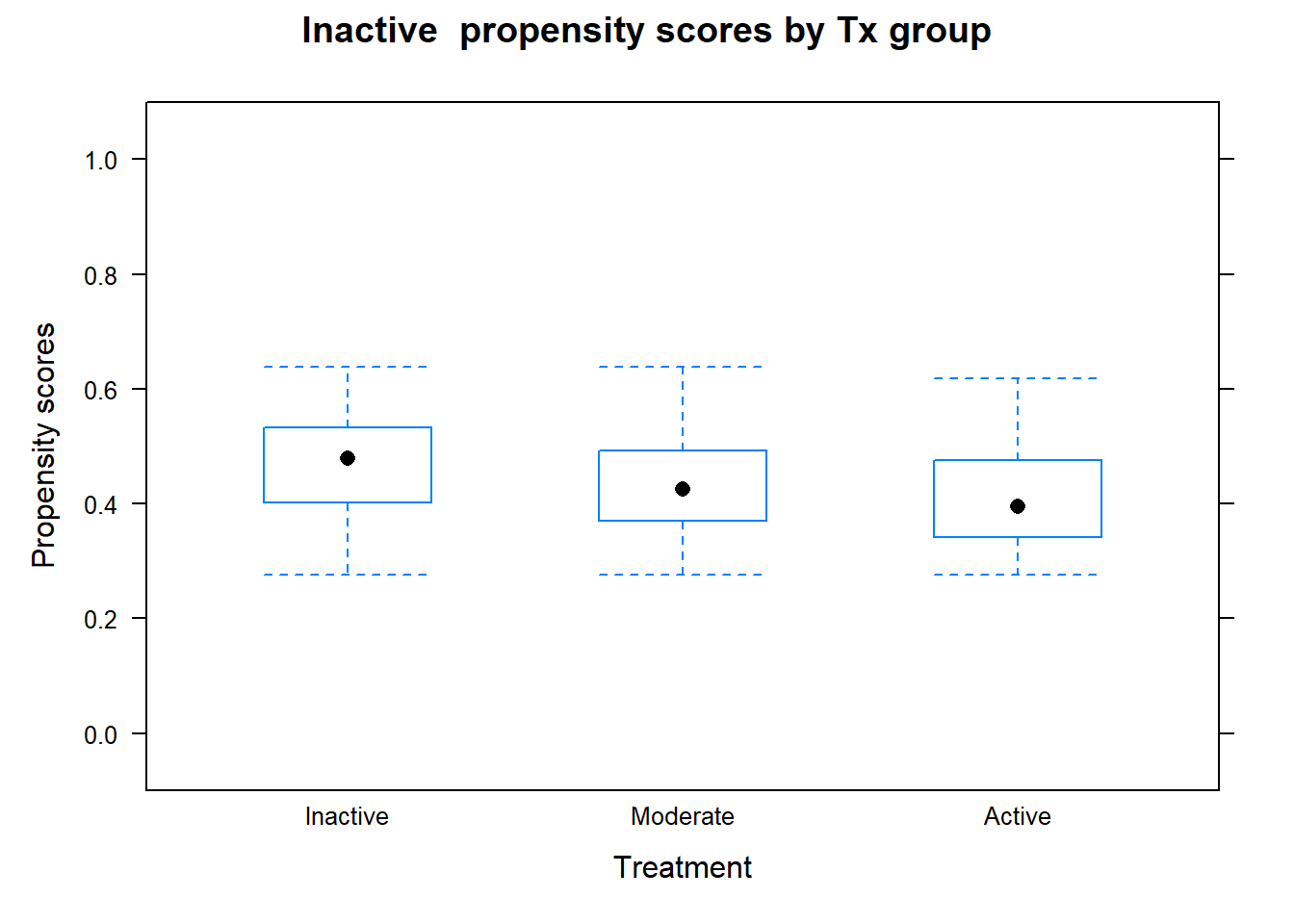
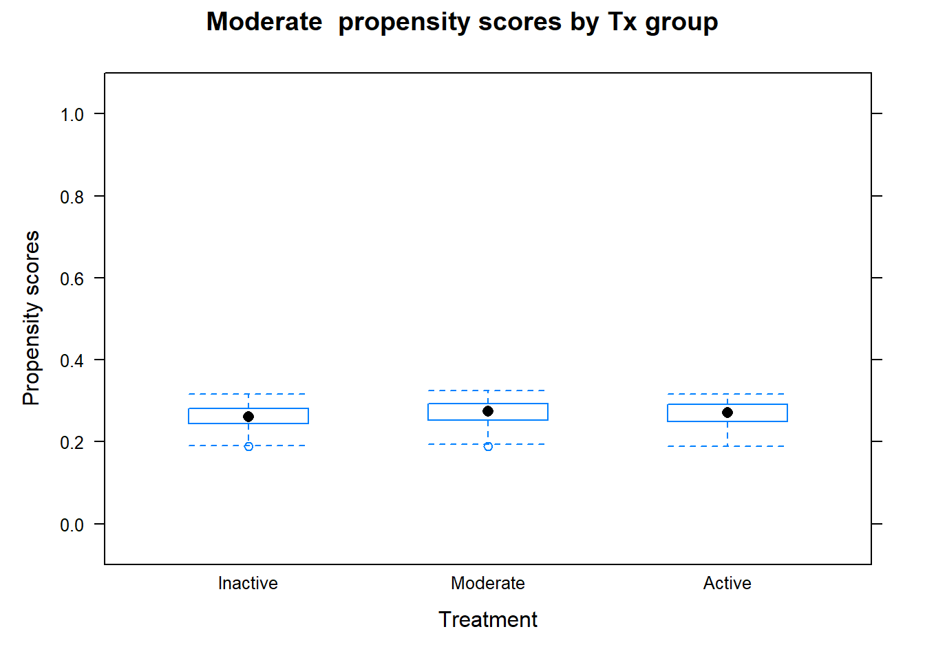
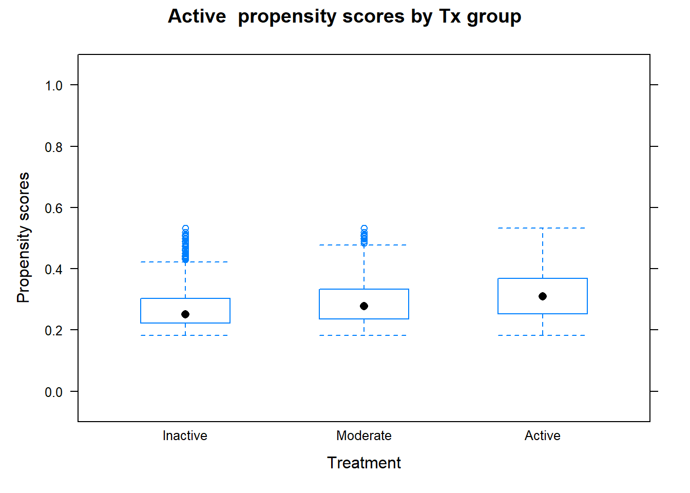
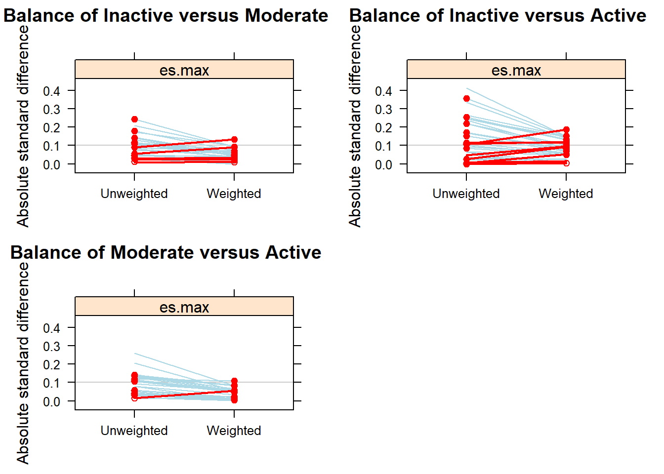
ps.fit3 <- mnps(ps.formula3, data = dat.analytic, estimand = "ATE", verbose = FALSE,
stop.method = c("es.max"), n.trees = 200, sampw = dat.analytic$weight)
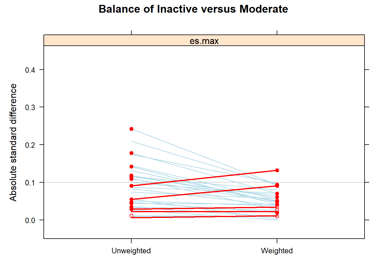
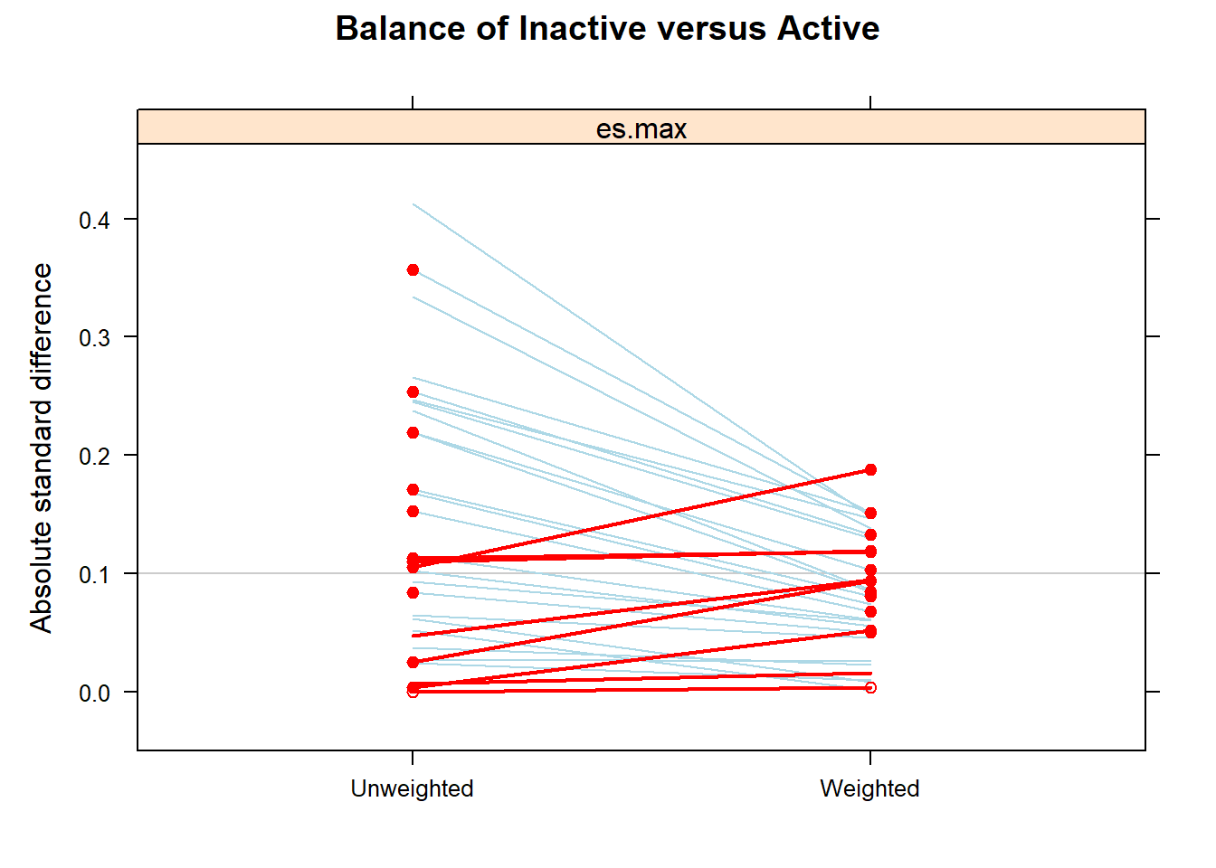
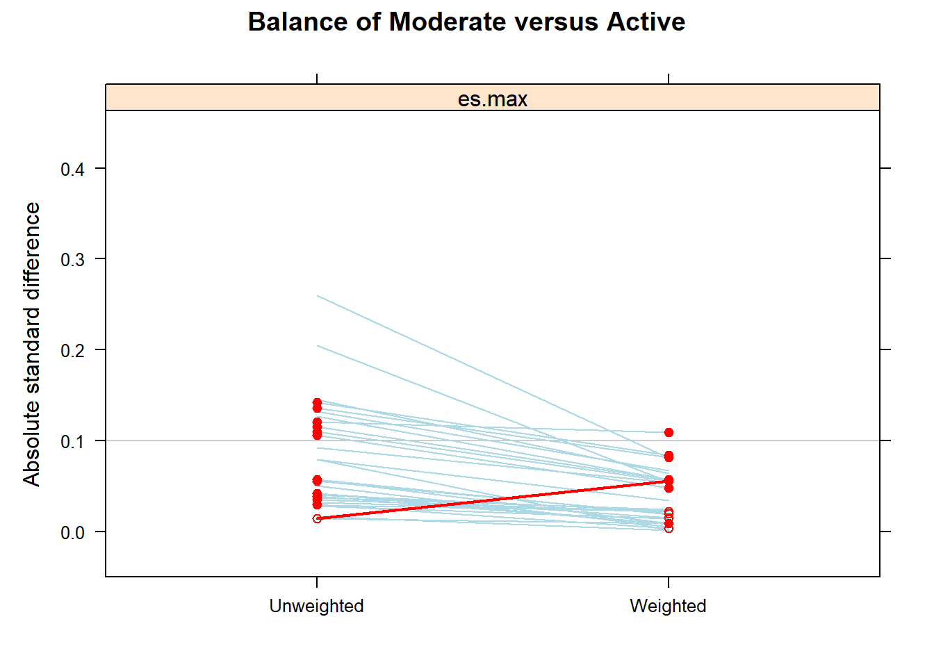
summary(ps.fit3)
#> Summary of pairwise comparisons:
#> max.std.eff.sz min.p max.ks min.ks.pval stop.method
#> 1 0.4134866 0 1 0 unw
#> 2 0.1880231 0 1 0 es.max
#>
#> Sample sizes and effective sample sizes:
#> treatment n ESS:es.max
#> 1 Inactive 17569 7361.137
#> 2 Moderate 10557 4875.807
#> 3 Active 11508 5376.500Creating weights
Let us create PS weights:
# IPW
dat.analytic$ipw3 <- ifelse(dat.analytic$phyact=="Active", 1/ps3$Active,
                           ifelse(dat.analytic$phyact=="Moderate", 1/ps3$Moderate,
                                  1/ps3$Inactive))
with(dat.analytic, by(ipw3, phyact, summary))
#> phyact: Inactive
#>    Min. 1st Qu.  Median    Mean 3rd Qu.    Max.
#>   1.565   1.877   2.086   2.206   2.484   3.624
#> ------------------------------------------------------------
#> phyact: Moderate
#>    Min. 1st Qu.  Median    Mean 3rd Qu.    Max.
#>   3.072   3.415   3.652   3.709   3.947   5.306
#> ------------------------------------------------------------
#> phyact: Active
#>    Min. 1st Qu.  Median    Mean 3rd Qu.    Max.
#>   1.876   2.716   3.229   3.320   3.952   5.465
Weights are not large compared to options 1 and 2.
Balance checking
Now, we will check the balance in terms of SMD:
library(survey)
vars <- c("age", "sex", "married", "race", "edu", "income", "bmi", "doctor", "stress",
          "smoke", "drink", "fruit", "bp", "diab", "OA", "immigrate")

# Design
w.design <- svydesign(id = ~1, weights = ~ipw3, data = dat.analytic)

# Table 1
tabw <- svyCreateTableOne(vars = vars, strata = "phyact", data = w.design, test = F)
print(tabw, smd = T, showAllLevels = T)
#>                Stratified by phyact
#>                 level             Inactive        Moderate
#>   n                               38763.2         39159.6
#>   age (%)       20-29 years        6086.5 (15.7)   6641.5 (17.0)
#>                 30-39 years        7624.6 (19.7)   8171.6 (20.9)
#>                 40-49 years        7057.4 (18.2)   7073.0 (18.1)
#>                 50-59 years        6267.5 (16.2)   5894.9 (15.1)
#>                 60-64 years        2399.6 ( 6.2)   2390.7 ( 6.1)
#>                 65 years and over  6883.8 (17.8)   5859.8 (15.0)
#>                 teen               2443.7 ( 6.3)   3128.1 ( 8.0)
#>   sex (%)       Female            20928.4 (54.0)  21097.6 (53.9)
#>                 Male              17834.8 (46.0)  18062.0 (46.1)
#>   married (%)   not single        21244.6 (54.8)  21279.5 (54.3)
#>                 single            17518.5 (45.2)  17880.1 (45.7)
#>   race (%)      Non-white          3683.4 ( 9.5)   3666.8 ( 9.4)
#>                 White             35079.7 (90.5)  35492.8 (90.6)
#>   edu (%)       < 2ndary           7610.9 (19.6)   6692.3 (17.1)
#>                 2nd grad.          7088.9 (18.3)   6693.3 (17.1)
#>                 Other 2nd grad.    3558.1 ( 9.2)   3619.6 ( 9.2)
#>                 Post-2nd grad.    20505.3 (52.9)  22154.2 (56.6)
#>   income (%)    $29,999 or less    9138.3 (23.6)   7750.6 (19.8)
#>                 $30,000-$49,999    8400.8 (21.7)   7956.3 (20.3)
#>                 $50,000-$79,999    9946.0 (25.7)  10696.8 (27.3)
#>                 $80,000 or more   11278.0 (29.1)  12755.9 (32.6)
#>   bmi (%)       Underweight        1195.7 ( 3.1)    967.7 ( 2.5)
#>                 healthy weight    16766.4 (43.3)  18791.6 (48.0)
#>                 Overweight        20801.0 (53.7)  19400.2 (49.5)
#>   doctor (%)    No                 5070.5 (13.1)   4827.3 (12.3)
#>                 Yes               33692.7 (86.9)  34332.3 (87.7)
#>   stress (%)    Not too stressed  29885.7 (77.1)  31099.5 (79.4)
#>                 stressed           8877.5 (22.9)   8060.0 (20.6)
#>   smoke (%)     Current smoker    10737.3 (27.7)   9401.4 (24.0)
#>                 Former smoker     15204.3 (39.2)  16211.3 (41.4)
#>                 Never smoker      12821.5 (33.1)  13546.9 (34.6)
#>   drink (%)     Current drinker   31123.7 (80.3)  33043.2 (84.4)
#>                 Former driker      5322.0 (13.7)   4301.7 (11.0)
#>                 Never drank        2317.5 ( 6.0)   1814.6 ( 4.6)
#>   fruit (%)     0-3 daily serving 10529.0 (27.2)   8996.8 (23.0)
#>                 4-6 daily serving 19466.5 (50.2)  19851.5 (50.7)
#>                 6+ daily serving   8767.6 (22.6)  10311.3 (26.3)
#>   bp (%)        No                31712.5 (81.8)  33335.5 (85.1)
#>                 Yes                7050.7 (18.2)   5824.1 (14.9)
#>   diab (%)      No                36326.4 (93.7)  37499.3 (95.8)
#>                 Yes                2436.8 ( 6.3)   1660.2 ( 4.2)
#>   OA (%)        Control           33060.8 (85.3)  34579.5 (88.3)
#>                 OA                 5702.3 (14.7)   4580.0 (11.7)
#>   immigrate (%) not immigrant     36812.8 (95.0)  37425.9 (95.6)
#>                 recent             1950.3 ( 5.0)   1733.7 ( 4.4)
#>                Stratified by phyact
#>                 Active          SMD
#>   n             38211.2
#>   age (%)        6567.9 (17.2)   0.145
#>                  8208.6 (21.5)
#>                  7313.3 (19.1)
#>                  5555.3 (14.5)
#>                  2186.9 ( 5.7)
#>                  4539.2 (11.9)
#>                  3840.0 (10.0)
#>   sex (%)       18441.4 (48.3)   0.077
#>                 19769.8 (51.7)
#>   married (%)   20012.7 (52.4)   0.033
#>                 18198.5 (47.6)
#>   race (%)       3397.2 ( 8.9)   0.014
#>                 34814.0 (91.1)
#>   edu (%)        6186.6 (16.2)   0.081
#>                  6159.6 (16.1)
#>                  3630.7 ( 9.5)
#>                 22234.2 (58.2)
#>   income (%)     6758.9 (17.7)   0.120
#>                  7420.8 (19.4)
#>                 10612.9 (27.8)
#>                 13418.7 (35.1)
#>   bmi (%)        1041.5 ( 2.7)   0.112
#>                 19648.4 (51.4)
#>                 17521.2 (45.9)
#>   doctor (%)     5001.8 (13.1)   0.015
#>                 33209.4 (86.9)
#>   stress (%)    30845.7 (80.7)   0.059
#>                  7365.5 (19.3)
#>   smoke (%)      8531.3 (22.3)   0.083
#>                 16200.7 (42.4)
#>                 13479.2 (35.3)
#>   drink (%)     32817.1 (85.9)   0.101
#>                  3703.9 ( 9.7)
#>                  1690.1 ( 4.4)
#>   fruit (%)      7924.2 (20.7)   0.120
#>                 19284.4 (50.5)
#>                 11002.5 (28.8)
#>   bp (%)        33698.1 (88.2)   0.120
#>                  4513.1 (11.8)
#>   diab (%)      36930.8 (96.6)   0.092
#>                  1280.4 ( 3.4)
#>   OA (%)        34640.5 (90.7)   0.110
#>                  3570.7 ( 9.3)
#>   immigrate (%) 36764.3 (96.2)   0.040
#>                  1446.8 ( 3.8)
All covariates are balanced in terms of SMD.

Outcome analysis
Now, we will fit the outcome model:
# Create an indicator variable in the full dataset
dat.full$ind <- 0
dat.full$ind[dat.full$ID %in% dat.analytic$ID] <- 1

# New weight = IPW * survey weight
dat.analytic$ATEweight3 <- with(dat.analytic, ipw3 * weight)

# New weight variable in the full dataset
dat.full$ATEweight3 <- 0
dat.full$ATEweight3[dat.full$ID %in% dat.analytic$ID] <- dat.analytic$ATEweight3

# Survey setup with full data
w.design0 <- svydesign(id = ~1, weights = ~ATEweight3, data = dat.full)

# Subset the design for analytic sample
w.design1 <- subset(w.design0, ind == 1)

# Weighted proportion
w.prop <- svyby(formula = ~CVD, by = ~phyact, design = w.design1, FUN = svymean)
w.propOther approches for multiple treatments
Not covered here, but possible to do in a multiple treatments context:
- Propensity score matching
- Propensity score stratification
- Marginal mean weighting