Exercise 3 Solution (A)
Exercise: Phased Multi-Year NHANES Data Wrangling
Instructions: Use the R programming language and functions from the tidyverse, nhanesA, tableone, and naniar packages to complete this exercise. We will build up our dataset in phases, starting with a single year and expanding to multiple survey cycles.
Please knit your final R Markdown file and submit the knitted HTML or PDF document ONLY.
Setup: Load Packages
First, run the following code block to ensure the required packages are installed and loaded into your R session.
Problem 1: Import and Translate Single-Year Data
Download the Demographic (DEMO) data for the 2013-2014 NHANES cycle, using translated = TRUE to automatically convert coded values into text labels.
# Download and translate the 2013-2014 demographic data
nhanes_demo_1314 <- nhanes("DEMO_H", translated = TRUE)
# Check the first few rows to see the translated values
head(nhanes_demo_1314[, c("SEQN", "RIAGENDR", "RIDAGEYR", "RIDRETH3")])
Problem 2: Add Body Measures Data for a Single Year
Download the Body Measures (BMX) data for the same 2013-2014 cycle and merge it with the demographic data from Problem 1.
# Download the 2013-2014 body measures data
nhanes_bmx_1314 <- nhanes("BMX_H", translated = TRUE)
# Merge the BMX data with the DEMO data from Problem 1
nhanes_1314_complete <- full_join(nhanes_demo_1314, nhanes_bmx_1314, by = "SEQN")
# Check the dimensions of the merged dataset
dim(nhanes_1314_complete)
#> [1] 10175    72
Problem 3: Import and Merge Multi-Cycle Data with Translation
Expand to multiple years, using translated = TRUE for all downloads. Merge both the Demographic (DEMO) and Body Measures (BMX) data for all three NHANES cycles: 2013-2014 (H), 2015-2016 (I), and 2017-2018 (J). Combine them into a single dataframe named nhanes_raw.
# Define the cycles to download
cycles <- c("H", "I", "J")
# Create a list to store data from each cycle
all_cycles_data <- list()
# Loop through each cycle, download with translation, and merge the data
for (cycle_code in cycles) {
  demo_data <- nhanes(paste0("DEMO_", cycle_code), translated = TRUE)
  bmx_data <- nhanes(paste0("BMX_", cycle_code), translated = TRUE)
  all_cycles_data[[cycle_code]] <- full_join(demo_data, bmx_data, by = "SEQN")
}
# Combine the data from all cycles into one dataframe
nhanes_raw <- bind_rows(all_cycles_data)
# Check the dimensions of the final raw dataset
dim(nhanes_raw)
#> [1] 29400    78
Problem 4: Data Cleaning and Filtering
Using the nhanes_raw dataset, we will now create our clean dataset. This involves filtering our population to adults and then creating our analysis variables.
- Filter for Adults: Keep only participants aged 20 years or older.
-
Rename Variables:
RIAGENDRtoSex,RIDAGEYRtoAge,RIDRETH3toRaceEthnicity,BMXBMItoBMI. -
Group
RaceEthnicity: Combine “Mexican American” and “Other Hispanic” into a single “Hispanic” category. -
Create
AgeGroup: CategorizeAgeinto “20-39”, “40-59”, and “60+”. -
Create
BMICat: CategorizeBMIinto “Underweight”, “Normal weight”, “Overweight”, and “Obese”.
nhanes_clean <- nhanes_raw %>%
  # Step 1: Filter the data to include only adults
  filter(RIDAGEYR >= 20) %>%
  # Step 2: Rename variables
  rename(
    Sex = RIAGENDR,
    Age = RIDAGEYR,
    RaceEthnicity = RIDRETH3,
    BMI = BMXBMI
  ) %>%
  # Create new variables
  mutate(
    # Step 3: Group the detailed race categories into broader ones
    RaceEthnicity = case_when(
      RaceEthnicity %in% c("Mexican American", "Other Hispanic") ~ "Hispanic",
      RaceEthnicity == "Non-Hispanic White" ~ "Non-Hispanic White",
      RaceEthnicity == "Non-Hispanic Black" ~ "Non-Hispanic Black",
      RaceEthnicity == "Non-Hispanic Asian" ~ "Non-Hispanic Asian",
      TRUE ~ "Other" # Groups "Other Race - Including Multi-Racial" and any NAs
    ),
    # Convert the new character RaceEthnicity to a factor with the desired level order
    RaceEthnicity = factor(RaceEthnicity,
                           levels = c("Non-Hispanic White", "Non-Hispanic Black", "Hispanic", "Non-Hispanic Asian", "Other")),

    # Step 4: Create AgeGroup (now without NAs because we filtered)
    AgeGroup = cut(Age,
                   breaks = c(19, 39, 59, Inf),
                   labels = c("20-39", "40-59", "60+"),
                   right = TRUE),

    # Step 5: Create BMICat
    BMICat = cut(BMI,
                 breaks = c(0, 18.5, 25, 30, Inf),
                 labels = c("Underweight", "Normal weight", "Overweight", "Obese"),
                 right = FALSE)
  )

# Check the structure to confirm variables are correct
str(nhanes_clean[, c("SEQN", "Sex", "Age", "AgeGroup", "RaceEthnicity", "BMI")])
#> 'data.frame':    17057 obs. of  6 variables:
#>  $ SEQN         : num  73557 73558 73559 73561 73562 ...
#>  $ Sex          : Factor w/ 2 levels "Male","Female": 1 1 1 2 1 2 1 2 1 2 ...
#>  $ Age          : num  69 54 72 73 56 61 42 56 65 26 ...
#>  $ AgeGroup     : Factor w/ 3 levels "20-39","40-59",..: 3 2 3 3 2 3 2 2 3 1 ...
#>  $ RaceEthnicity: Factor w/ 5 levels "Non-Hispanic White",..: 2 1 1 1 3 1 3 1 1 1 ...
#>  $ BMI          : num  26.7 28.6 28.9 19.7 41.7 35.7 NA 26.5 22 20.3 ...
Problem 5: Create Final Analytic Dataset
Create a final, analysis-ready dataset named nhanes_analysis that includes only the key variables.
nhanes_analysis <- select(nhanes_clean, SEQN, Sex, Age, AgeGroup, RaceEthnicity, BMI, BMICat)

# Display the structure of the final analytic dataset
str(nhanes_analysis)
#> 'data.frame':    17057 obs. of  7 variables:
#>  $ SEQN         : num  73557 73558 73559 73561 73562 ...
#>  $ Sex          : Factor w/ 2 levels "Male","Female": 1 1 1 2 1 2 1 2 1 2 ...
#>  $ Age          : num  69 54 72 73 56 61 42 56 65 26 ...
#>  $ AgeGroup     : Factor w/ 3 levels "20-39","40-59",..: 3 2 3 3 2 3 2 2 3 1 ...
#>  $ RaceEthnicity: Factor w/ 5 levels "Non-Hispanic White",..: 2 1 1 1 3 1 3 1 1 1 ...
#>  $ BMI          : num  26.7 28.6 28.9 19.7 41.7 35.7 NA 26.5 22 20.3 ...
#>  $ BMICat       : Factor w/ 4 levels "Underweight",..: 3 3 3 2 4 4 NA 3 2 2 ...
Problem 6: Investigate Missing Data
Now that our data is correctly filtered and processed, let’s re-examine the missing data patterns. The missingness should be much lower.
# 1. Count missing values for each column
missing_counts <- colSums(is.na(nhanes_analysis))
print(missing_counts)
#>          SEQN           Sex           Age      AgeGroup RaceEthnicity
#>             0             0             0             0             0
#>           BMI        BMICat
#>           956           956

# 2. Visualize the missing data
gg_miss_var(nhanes_analysis, show_pct = TRUE) +
  labs(title = "Missing Data in NHANES Adult Participants (2013-2018)")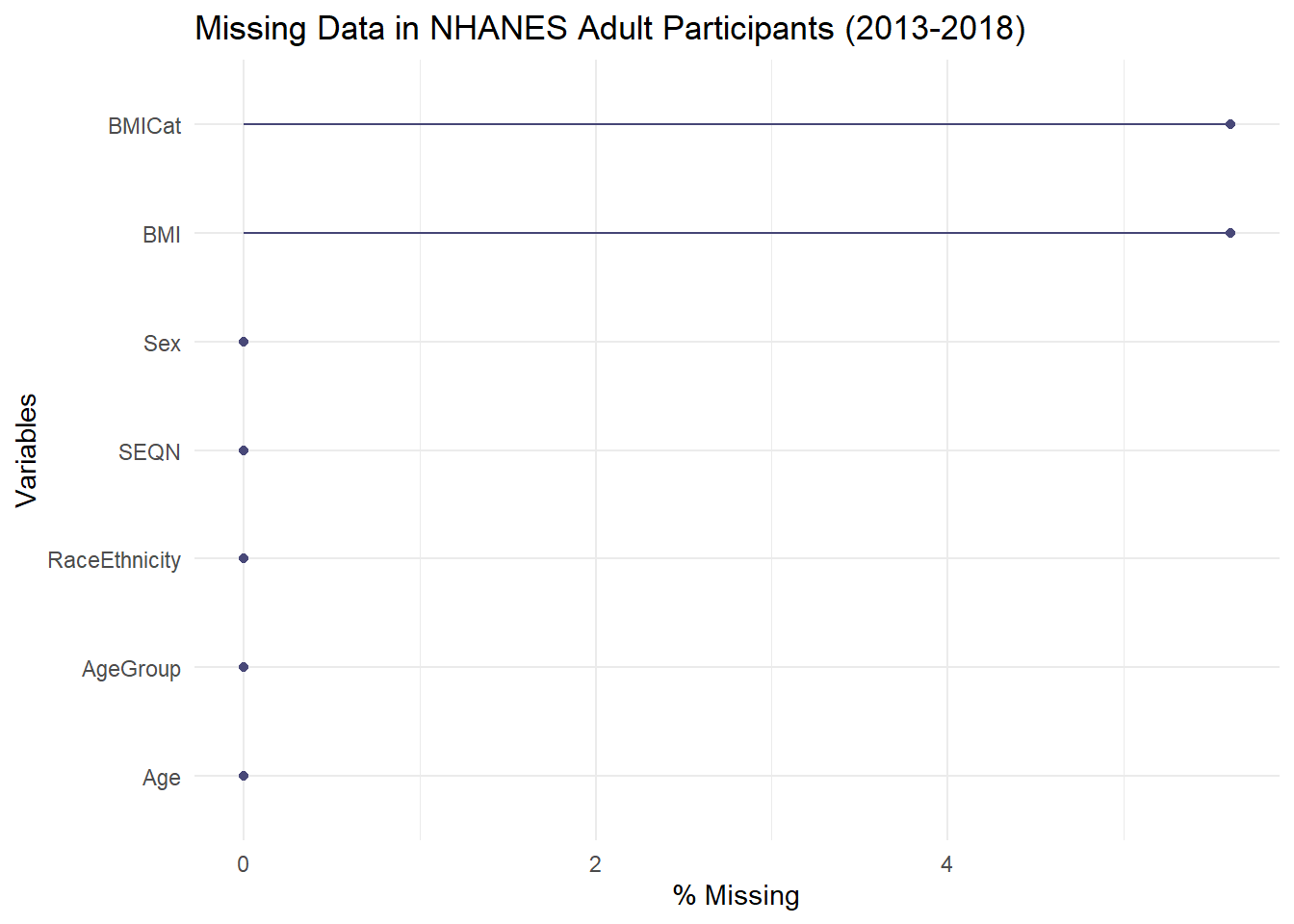
Problem 7: Create a Descriptive Table
Finally, with the data correctly loaded and cleaned for our adult population, create the summary table of sample characteristics, stratified by Sex.
# Define the variables for the table
vars <- c("Age", "AgeGroup", "RaceEthnicity", "BMI", "BMICat")

# Create the table, stratified by Sex
tab1 <- CreateTableOne(vars = vars, data = nhanes_analysis, strata = "Sex", addOverall = TRUE, test = FALSE)

# Print the table, showing all levels and missing data counts
print(tab1, smd = FALSE, showAllLevels = TRUE, missing = TRUE)
#>                    Stratified by Sex
#>                     level              Overall       Male
#>   n                                    17057          8207
#>   Age (mean (SD))                      50.03 (17.74) 50.23 (17.83)
#>   AgeGroup (%)      20-39               5594 (32.8)   2687 (32.7)
#>                     40-59               5571 (32.7)   2612 (31.8)
#>                     60+                 5892 (34.5)   2908 (35.4)
#>   RaceEthnicity (%) Non-Hispanic White  6270 (36.8)   3094 (37.7)
#>                     Non-Hispanic Black  3673 (21.5)   1759 (21.4)
#>                     Hispanic            4290 (25.2)   1978 (24.1)
#>                     Non-Hispanic Asian  2168 (12.7)   1034 (12.6)
#>                     Other                656 ( 3.8)    342 ( 4.2)
#>   BMI (mean (SD))                      29.49 (7.21)  28.93 (6.33)
#>   BMICat (%)        Underweight          247 ( 1.5)    105 ( 1.4)
#>                     Normal weight       4244 (26.4)   1966 (25.5)
#>                     Overweight          5168 (32.1)   2853 (37.0)
#>                     Obese               6442 (40.0)   2790 (36.2)
#>                    Stratified by Sex
#>                     Female        Missing
#>   n                  8850
#>   Age (mean (SD))   49.86 (17.66) 0.0
#>   AgeGroup (%)       2907 (32.8)  0.0
#>                      2959 (33.4)
#>                      2984 (33.7)
#>   RaceEthnicity (%)  3176 (35.9)  0.0
#>                      1914 (21.6)
#>                      2312 (26.1)
#>                      1134 (12.8)
#>                       314 ( 3.5)
#>   BMI (mean (SD))   30.01 (7.90)  5.6
#>   BMICat (%)          142 ( 1.7)  5.6
#>                      2278 (27.2)
#>                      2315 (27.6)
#>                      3652 (43.5)