Mixed effects models

In this section, we will learn about mixed effects models. Mixed effects models are popular choices for modeling repeated measurements, such as longitudinal or clustered data. Examples of longitudinal data include blood pressure measurements taken over time from the same individuals and CD4 count over time from the same individuals. Examples of clustered data include students within schools and patients within hospitals. There are two components in a mixed effects model: fixed effects and random effects:

Fixed effects refer to general trends that are applicable to all subjects/clusters. This implies that we might want to investigate how students perform (on average) in different subjects such as math and history. These effects are commonly observed, i.e., fixed, across all schools.
Random Effects capture the unique characteristics of each subject/cluster that differentiate them from one another. For instance, some schools may have better resources, more experienced teachers, or a more supportive learning environment. These differences are specific to each school, and we use random effects to capture them.

# Load required packages
knitr::opts_chunk$set(echo = TRUE)
require(kableExtra)
require(Matrix)
require(jtools)

Repeated measures

A useful reference on repeated measures is Section 9.2 of Faraway (2016).

In repeated measurement design, the response variable are measured multiple times for each individuals.

Linear Mixed Effects Models for Repeated Measures Data

A useful reference on linear mixed effects models is Section 12.4 of Hothorn and Everitt (2014).

Important

The linear mixed effect models are based on the idea that the correlation of an individual’s responses depends on some unobserved individual characteristics.
In linear mixed effect models, we treat these unobserved characteristics as random effects in our model. If we could conditional on the random effects, then the repeated measurements can be assumed to be independent.

Data

We are going to use the BtheB dataset from the HSAUR2 package to explain the linear mixed effect model:

library(HSAUR2)
data("BtheB")
kable(head(BtheB))%>%
  kable_styling(bootstrap_options = "striped", full_width = F, 
                position = "left")

drug	length	treatment	bdi.pre	bdi.2m	bdi.3m	bdi.5m	bdi.8m
No	>6m	TAU	29	2	2	NA	NA
Yes	>6m	BtheB	32	16	24	17	20
Yes	<6m	TAU	25	20	NA	NA	NA
No	>6m	BtheB	21	17	16	10	9
Yes	>6m	BtheB	26	23	NA	NA	NA
Yes	<6m	BtheB	7	0	0	0	0

A typical form of repeated measurement data from a clinical trial data.
The individuals are allocated to different treatments then the response Beck Depression Inventory II were taken at baseline, 2, 3, 5, and 8 months

## Box-plot of responses at different time points in treatment and control groups
data("BtheB", package = "HSAUR2")
layout(matrix(1:2, nrow = 1))
ylim <- range(BtheB[,grep("bdi", names(BtheB))],na.rm = TRUE)
tau <- subset(BtheB, treatment == "TAU")[, grep("bdi", names(BtheB))]
boxplot(tau, main = "Treated as Usual", ylab = "BDI",
        xlab = "Time (in months)", 
        names = c(0, 2, 3, 5, 8),ylim = ylim)
btheb <- subset(BtheB, treatment == "BtheB")[, grep("bdi", names(BtheB))]
boxplot(btheb, main = "Beat the Blues", ylab = "BDI",
        xlab = "Time (in months)", 
        names = c(0, 2, 3, 5, 8),ylim = ylim)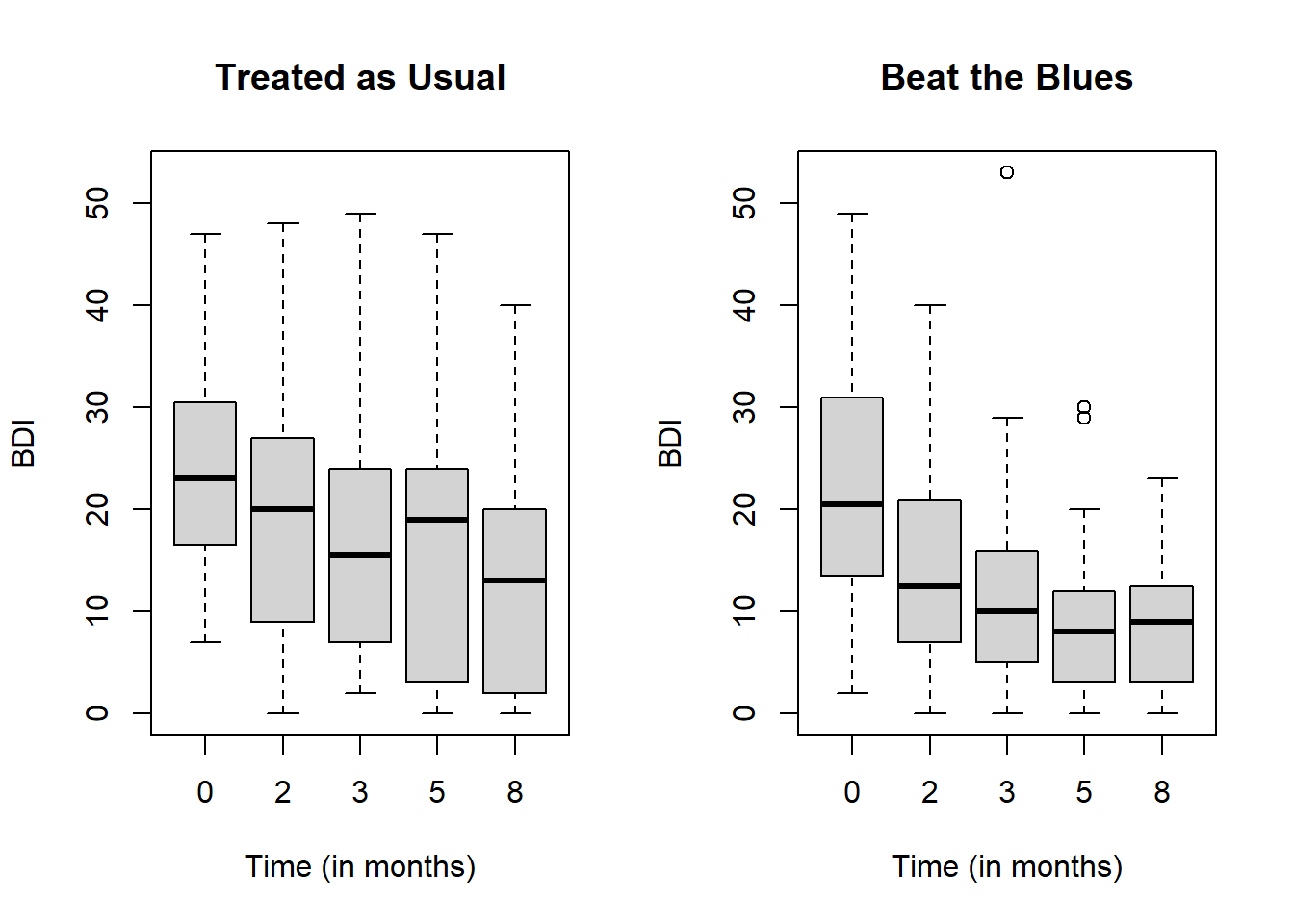

The side-by-side box plots show the distributions of BDI overtime between control (Treated as Usual) and intervention (Beat the Blues) groups.
As time goes, drops in BDI are more obvious in intervention which may indicate the intervention is effective.

Regular model fixed intercept and slope

To compare, we start with fixed effect linear model, i.e., a regular linear model without any random effect:

## To analyze the data, we first need to convert the dataset to a analysis-ready form
BtheB$subject <- factor(rownames(BtheB))
nobs <- nrow(BtheB)
BtheB_long <- reshape(BtheB, idvar = "subject", 
                      varying = c("bdi.2m", "bdi.3m", "bdi.5m", 
                                  "bdi.8m"), 
                      direction = "long")
BtheB_long$time <- rep(c(2, 3, 5, 8), rep(nobs, 4))
kable(head(BtheB_long))%>%
  kable_styling(bootstrap_options = "striped", full_width = F, 
                position = "left")

	drug	length	treatment	bdi.pre	subject	time	bdi
1.2m	No	>6m	TAU	29	1	2	2
2.2m	Yes	>6m	BtheB	32	2	2	16
3.2m	Yes	<6m	TAU	25	3	2	20
4.2m	No	>6m	BtheB	21	4	2	17
5.2m	Yes	>6m	BtheB	26	5	2	23
6.2m	Yes	<6m	BtheB	7	6	2	0

unique(BtheB_long$subject)
#>   [1] 1   2   3   4   5   6   7   8   9   10  11  12  13  14  15  16  17  18 
#>  [19] 19  20  21  22  23  24  25  26  27  28  29  30  31  32  33  34  35  36 
#>  [37] 37  38  39  40  41  42  43  44  45  46  47  48  49  50  51  52  53  54 
#>  [55] 55  56  57  58  59  60  61  62  63  64  65  66  67  68  69  70  71  72 
#>  [73] 73  74  75  76  77  78  79  80  81  82  83  84  85  86  87  88  89  90 
#>  [91] 91  92  93  94  95  96  97  98  99  100
#> 100 Levels: 1 10 100 11 12 13 14 15 16 17 18 19 2 20 21 22 23 24 25 26 27 ... 99
kable(subset(BtheB_long,  subject == 2))%>%
  kable_styling(bootstrap_options = "striped", full_width = F, 
                position = "left")

	drug	length	treatment	bdi.pre	subject	time	bdi
2.2m	Yes	>6m	BtheB	32	2	2	16
2.3m	Yes	>6m	BtheB	32	2	3	24
2.5m	Yes	>6m	BtheB	32	2	5	17
2.8m	Yes	>6m	BtheB	32	2	8	20

kable(subset(BtheB_long,  subject == 99))%>%
  kable_styling(bootstrap_options = "striped", full_width = F, 
                position = "left")

	drug	length	treatment	bdi.pre	subject	time	bdi
99.2m	No	<6m	TAU	13	99	2	5
99.3m	No	<6m	TAU	13	99	3	5
99.5m	No	<6m	TAU	13	99	5	0
99.8m	No	<6m	TAU	13	99	8	6



lmfit <- lm(bdi ~ bdi.pre + time + treatment + drug +length, 
            data = BtheB_long, na.action = na.omit)
require(jtools)
summ(lmfit)

Observations	280 (120 missing obs. deleted)
Dependent variable	bdi
Type	OLS linear regression

F(5,274)	35.78
R²	0.40
Adj. R²	0.38

	Est.	S.E.	t val.	p
(Intercept)	7.32	1.73	4.24	0.00
bdi.pre	0.57	0.05	10.44	0.00
time	-0.94	0.24	-3.97	0.00
treatmentBtheB	-3.32	1.10	-3.02	0.00
drugYes	-3.57	1.15	-3.11	0.00
length>6m	1.71	1.11	1.54	0.12
Standard errors: OLS

Random intercept but fixed slope

Let us start with a model with a random intercept but fixed slope. In this case, the resulting regression line for each individual is parallel (for fixed slope) but have different intercepts (for random intercept).

## Fit a random intercept model with lme4 package
library("lme4")
BtheB_lmer1 <- lmer(bdi ~ bdi.pre + time + treatment + drug +length 
                    + (1 | subject), data = BtheB_long, 
                    REML = FALSE, na.action = na.omit)

summary(BtheB_lmer1)
#> Linear mixed model fit by maximum likelihood  ['lmerMod']
#> Formula: bdi ~ bdi.pre + time + treatment + drug + length + (1 | subject)
#>    Data: BtheB_long
#> 
#>      AIC      BIC   logLik deviance df.resid 
#>   1887.5   1916.6   -935.7   1871.5      272 
#> 
#> Scaled residuals: 
#>     Min      1Q  Median      3Q     Max 
#> -2.6975 -0.5026 -0.0638  0.4124  3.8203 
#> 
#> Random effects:
#>  Groups   Name        Variance Std.Dev.
#>  subject  (Intercept) 48.78    6.984   
#>  Residual             25.14    5.014   
#> Number of obs: 280, groups:  subject, 97
#> 
#> Fixed effects:
#>                Estimate Std. Error t value
#> (Intercept)     5.59239    2.24244   2.494
#> bdi.pre         0.63968    0.07789   8.212
#> time           -0.70476    0.14639  -4.814
#> treatmentBtheB -2.32908    1.67036  -1.394
#> drugYes        -2.82495    1.72684  -1.636
#> length>6m       0.19708    1.63832   0.120
#> 
#> Correlation of Fixed Effects:
#>             (Intr) bdi.pr time   trtmBB drugYs
#> bdi.pre     -0.682                            
#> time        -0.238  0.020                     
#> tretmntBthB -0.390  0.121  0.018              
#> drugYes     -0.073 -0.237 -0.022 -0.323       
#> length>6m   -0.243 -0.242 -0.036  0.002  0.157
summ(BtheB_lmer1)

Observations	280
Dependent variable	bdi
Type	Mixed effects linear regression

AIC	1887.49
BIC	1916.57
Pseudo-R² (fixed effects)	0.39
Pseudo-R² (total)	0.79

Fixed Effects
	Est.	S.E.	t val.	d.f.	p
(Intercept)	5.59	2.24	2.49	108.98	0.01
bdi.pre	0.64	0.08	8.21	104.08	0.00
time	-0.70	0.15	-4.81	199.32	0.00
treatmentBtheB	-2.33	1.67	-1.39	97.12	0.17
drugYes	-2.82	1.73	-1.64	98.20	0.11
length>6m	0.20	1.64	0.12	100.26	0.90
p values calculated using Satterthwaite d.f.

Random Effects
Group	Parameter	Std. Dev.
subject	(Intercept)	6.98
Residual		5.01

Grouping Variables
Group	# groups	ICC
subject	97	0.66

Important

AIC, BIC, and -loglik etc are goodness-of-fit statistics, which tells you how well the model fits your data. Since there is no standard to tell what values of these statistics are good, without comparison with other models, they have little information to tell.
Fixed effects: this is the standard output we will have in any fixed-effect model. The interpretation of estimated coefficients will be similar to a regular linear model.
You may compare the outputs with the regular linear model, then you will find that lm tends to underestimate the SE for estimated coefficients.

library(ggplot2)
BtheB_longna <- na.omit(BtheB_long)
dat <- data.frame(time=BtheB_longna$time,pred=fitted(BtheB_lmer1),
                  Subject= BtheB_longna$subject)
ggplot(data=dat,aes(x=time, y=pred, group=Subject, 
                    color=Subject)) + theme_classic() +
    geom_line()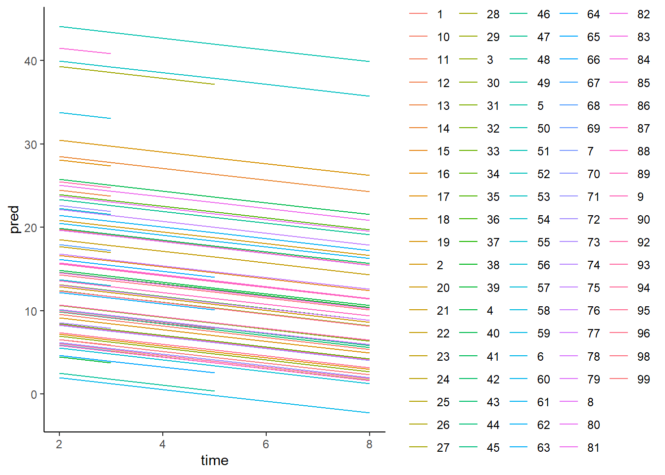

As we can see, for each individual, we have different intercepts but the slope over follow-up time is the same. Next, we will fit the model with random intercept and random slope.

Random intercept and random slope

In the codes below, we fitted a mixed effects model with both random intercept and random slope:

## We can fit a random slope and intercept model using lme4 package and treat variable time as random slope. 
library("lme4")
BtheB_lmer2 <- lmer(bdi ~ bdi.pre + time + treatment + drug +length + 
                   (time | subject), data = BtheB_long, REML = FALSE, 
                   na.action = na.omit)

summ(BtheB_lmer2)

Observations	280
Dependent variable	bdi
Type	Mixed effects linear regression

AIC	1891.04
BIC	1927.39
Pseudo-R² (fixed effects)	0.39
Pseudo-R² (total)	0.80

Fixed Effects
	Est.	S.E.	t val.	d.f.	p
(Intercept)	5.61	2.25	2.50	106.79	0.01
bdi.pre	0.64	0.08	8.25	102.78	0.00
time	-0.70	0.15	-4.56	57.69	0.00
treatmentBtheB	-2.38	1.67	-1.42	97.12	0.16
drugYes	-2.87	1.73	-1.66	98.18	0.10
length>6m	0.14	1.64	0.09	100.04	0.93
p values calculated using Satterthwaite d.f.

Random Effects
Group	Parameter	Std. Dev.
subject	(Intercept)	7.12
subject	time	0.43
Residual		4.90

Grouping Variables
Group	# groups	ICC
subject	97	0.68

The interpretation of the model outputs will be similar to the model with only random intercepts. Let us plot the data:

library(ggplot2)
BtheB_longna <- na.omit(BtheB_long)
dat <- data.frame(time=BtheB_longna$time,pred=fitted(BtheB_lmer2),
                  Subject= BtheB_longna$subject)
ggplot(data=dat,aes(x=time, y=pred, group=Subject, color=Subject)) + 
  theme_classic() +
    geom_line()

From the figure, we can see, we have different intercepts and different slopes over follow-up time for each individual.

Choice among models

A common question is to ask should I add random slope to our model or random intercept is good enough. We may want to compare the models in terms of AIC and BIC. Smaller values indicate a better model.

lm usually will not be considered as a competitor of lme as they basically apply to different types of data.
When choosing between random intercept and random slope, a quick solution is to fit all possible models then do likelihood ratio tests.
For example, I am not sure whether I should use random intercept only or random intercept + random slope. I could fit both model, then do a likelihood ratio test:

anova(BtheB_lmer1, BtheB_lmer2)

## The non-significant p-value shows that the second model is not 
## statistically different from the first model. Therefore, adding a 
## random slope is not necessary

The p-value is greater than 0.05, which indicate that adding a random slope does not make the fitting significantly better. To keep the model simple, we may just use random intercept.

Prediction of Random Effects

Ref: (Hothorn and Everitt 2014) Section 12.5

If you have noticed in the R output of linear mixed effect model. Random effects are not estimated in the model.

We could use the fitted model to predict random effects.
Also, the predicted random effects can be used to examine the assumptions we have for linear mixed effect model.

The ranef function is used to predict the random effect in R

qint <- ranef(BtheB_lmer1)$subject[["(Intercept)"]]
qint
#>  [1] -16.36173411  -2.44276827  -3.81655251   3.05333928   3.45142248
#>  [6]   7.76598376   2.72263773  -7.22484569   6.84680617  -1.02552084
#> [11]   2.40417048   1.16611114  -8.55346533  -6.25844483  -2.26117896
#> [16]  -5.23031336   2.52509381  -1.64263857  -1.07523649   3.93689163
#> [21]   7.66903473 -16.38156595   1.74883174  -1.31871410  -9.02883854
#> [26]  -2.75150756   2.38884151   2.72740404  -3.41918542   6.27519245
#> [31]  -4.52154811  -8.67437225  -0.34470208  -0.63972054  -0.08927194
#> [36]   7.61914282   2.91050412  -2.58455318   4.24637616 -16.01664364
#> [41]   5.90993779   3.21014012  -7.04631398   3.09608824   4.71327710
#> [46]  16.70161338   2.26241522   2.26584476  15.77002952   1.75410838
#> [51]   6.18741474   1.99791717   0.56774362   4.04107968  10.72891321
#> [56]  -1.54551028  -5.28330207   2.04552526   2.36472056  -1.56879952
#> [61]   6.63565636   5.45929329  -4.19695096  -6.39632488  -2.21496288
#> [66]  -0.95956136  -3.96021851   7.17628718  -1.41644518  -4.99763144
#> [71]  -2.83374092  -1.28015494   8.79345988  -0.33213428   1.43146353
#> [76]  -3.13316295  -6.52989461   2.51445573   5.93415004   3.42003755
#> [81]   4.49954804   3.75178702  -6.44832897  12.88173218  -9.36110814
#> [86]   2.02028152 -18.09960241  -6.53428535   5.06613705  -3.31816912
#> [91]   7.26187445   0.03103101  -8.14350181  -4.89326763   2.92437698
#> [96]   5.24835927  -5.96778945
## predict random effects using the fitted model

Check assumptions

Remember, we have two assumptions in the linear mixed effect model with random intercept:

error term follows normal distribution
beta for subject \(i\) follows normal distribution

We have predict the values of random effect and we could extract residuals from the fitted model. Therefore, we can use QQ-plot to check their normality

# Assumption 1
qres <- residuals(BtheB_lmer1)
qqnorm(qres, xlim = c(-3, 3), ylim = c(-20, 20), 
       ylab = "Estimated residuals",
       main = "Residuals")
qqline(qres)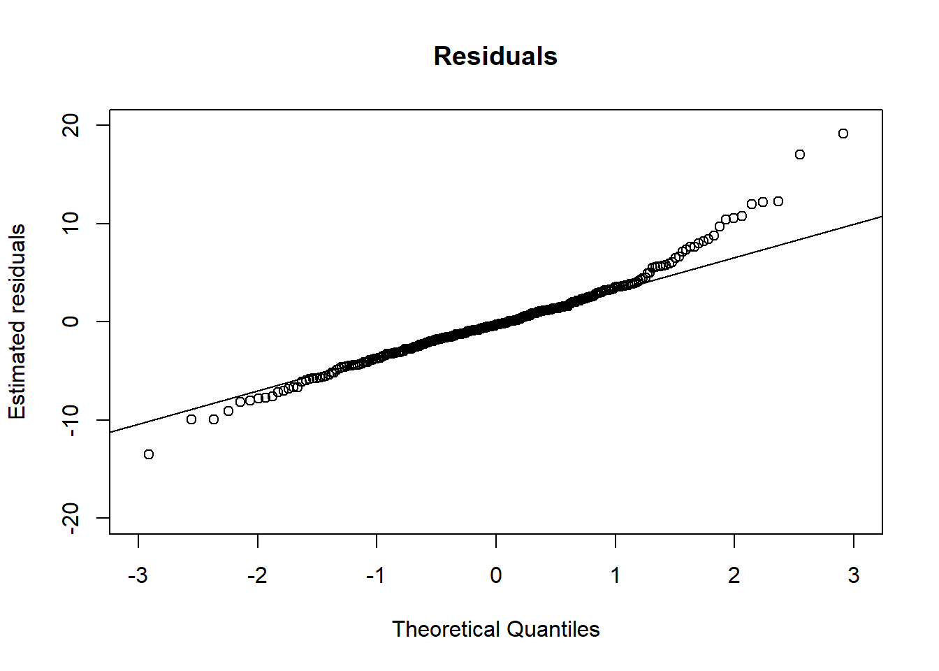


# Assumption 2
qint <- ranef(BtheB_lmer1)$subject[["(Intercept)"]]
qqnorm(qint, ylab = "Estimated random intercepts", 
       xlim = c(-3, 3), ylim = c(-20, 20),
       main = "Random intercepts")
qqline(qint)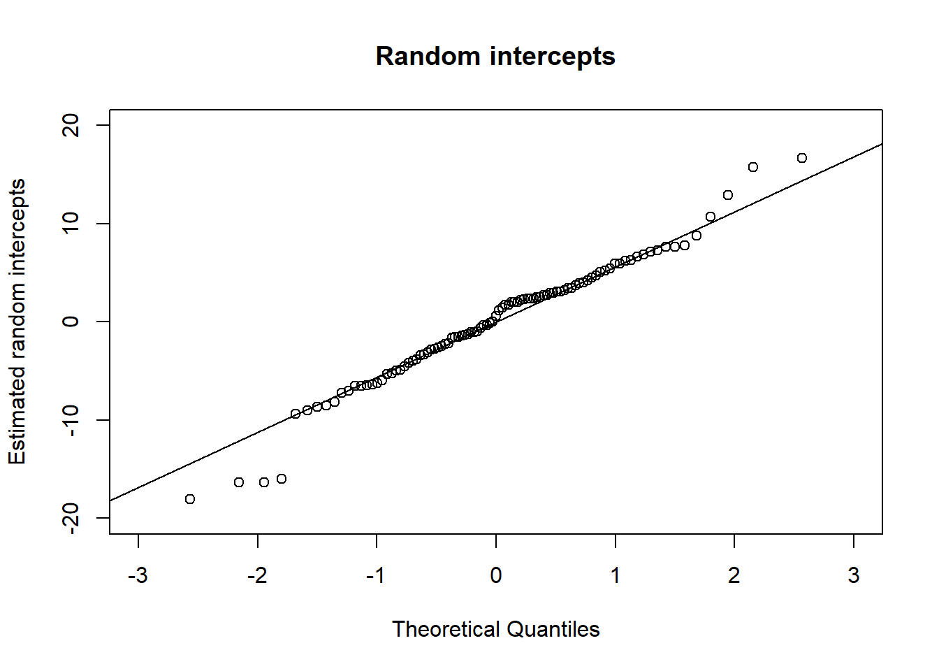

Since points are almost on the lines, we can say that the normality assumption is met.

Video content (optional)

Tip

For those who prefer a video walkthrough, feel free to watch the video below, which offers a description of an earlier version of the above content.

Reference

Faraway, Julian J. 2016. Extending the linear model with R: generalized linear, mixed effects and nonparametric regression models. CRC press.

Hothorn, Torsten, and Brian S Everitt. 2014. A Handbook of Statistical Analyses Using r. CRC press.