Continuous outcome
Important
This tutorial is very similar to one of the previous tutorials, but uses a different data (we used RHC data here). We are revisiting concepts related to prediction before introducing ideas related to machine learning.
In this chapter, we will talk about Regression that deals with prediction of continuous outcomes. We will use multiple linear regression to build the first prediction model.
Load dataset
Prediction for length of stay
Now, we show the regression fitting when outcome is continuous (length of stay).
Variables
baselinevars <- names(dplyr::select(ObsData,
                         !c(Length.of.Stay,Death)))
baselinevars
#>  [1] "Disease.category"      "Cancer"                "Cardiovascular"
#>  [4] "Congestive.HF"         "Dementia"              "Psychiatric"
#>  [7] "Pulmonary"             "Renal"                 "Hepatic"
#> [10] "GI.Bleed"              "Tumor"                 "Immunosupperssion"
#> [13] "Transfer.hx"           "MI"                    "age"
#> [16] "sex"                   "edu"                   "DASIndex"
#> [19] "APACHE.score"          "Glasgow.Coma.Score"    "blood.pressure"
#> [22] "WBC"                   "Heart.rate"            "Respiratory.rate"
#> [25] "Temperature"           "PaO2vs.FIO2"           "Albumin"
#> [28] "Hematocrit"            "Bilirubin"             "Creatinine"
#> [31] "Sodium"                "Potassium"             "PaCo2"
#> [34] "PH"                    "Weight"                "DNR.status"
#> [37] "Medical.insurance"     "Respiratory.Diag"      "Cardiovascular.Diag"
#> [40] "Neurological.Diag"     "Gastrointestinal.Diag" "Renal.Diag"
#> [43] "Metabolic.Diag"        "Hematologic.Diag"      "Sepsis.Diag"
#> [46] "Trauma.Diag"           "Orthopedic.Diag"       "race"
#> [49] "income"                "RHC.use"
Model
out.formula1
#> Length.of.Stay ~ Disease.category + Cancer + Cardiovascular +
#>     Congestive.HF + Dementia + Psychiatric + Pulmonary + Renal +
#>     Hepatic + GI.Bleed + Tumor + Immunosupperssion + Transfer.hx +
#>     MI + age + sex + edu + DASIndex + APACHE.score + Glasgow.Coma.Score +
#>     blood.pressure + WBC + Heart.rate + Respiratory.rate + Temperature +
#>     PaO2vs.FIO2 + Albumin + Hematocrit + Bilirubin + Creatinine +
#>     Sodium + Potassium + PaCo2 + PH + Weight + DNR.status + Medical.insurance +
#>     Respiratory.Diag + Cardiovascular.Diag + Neurological.Diag +
#>     Gastrointestinal.Diag + Renal.Diag + Metabolic.Diag + Hematologic.Diag +
#>     Sepsis.Diag + Trauma.Diag + Orthopedic.Diag + race + income +
#>     RHC.use
adj.fit1
Design Matrix
- Notations
- n is number of observations
- p is number of covariates
Expands factors to a set of dummy variables.
head(model.matrix(fit1))
#>   (Intercept) Disease.categoryCHF Disease.categoryOther Disease.categoryMOSF
#> 1           1                   0                     1                    0
#> 2           1                   0                     0                    1
#> 3           1                   0                     0                    1
#> 4           1                   0                     0                    0
#> 5           1                   0                     0                    1
#> 6           1                   0                     1                    0
#>   CancerLocalized (Yes) CancerMetastatic Cardiovascular1 Congestive.HF1
#> 1                     1                0               0              0
#> 2                     0                0               1              1
#> 3                     1                0               0              0
#> 4                     0                0               0              0
#> 5                     0                0               0              0
#> 6                     0                0               0              1
#>   Dementia1 Psychiatric1 Pulmonary1 Renal1 Hepatic1 GI.Bleed1 Tumor1
#> 1         0            0          1      0        0         0      1
#> 2         0            0          0      0        0         0      0
#> 3         0            0          0      0        0         0      1
#> 4         0            0          0      0        0         0      0
#> 5         0            0          0      0        0         0      0
#> 6         0            0          1      0        0         0      0
#>   Immunosupperssion1 Transfer.hx1 MI1 age[50,60) age[60,70) age[70,80)
#> 1                  0            0   0          0          0          1
#> 2                  1            1   0          0          0          1
#> 3                  1            0   0          0          0          0
#> 4                  1            0   0          0          0          1
#> 5                  0            0   0          0          1          0
#> 6                  0            0   0          0          0          0
#>   age[80, Inf) sexFemale       edu DASIndex APACHE.score Glasgow.Coma.Score
#> 1            0         0 12.000000 23.50000           46                  0
#> 2            0         1 12.000000 14.75195           50                  0
#> 3            0         1 14.069916 18.13672           82                  0
#> 4            0         1  9.000000 22.92969           48                  0
#> 5            0         0  9.945259 21.05078           72                 41
#> 6            1         1  8.000000 17.50000           38                  0
#>   blood.pressure         WBC Heart.rate Respiratory.rate Temperature
#> 1             41 22.09765620        124               10    38.69531
#> 2             63 28.89843750        137               38    38.89844
#> 3             57  0.04999542        130               40    36.39844
#> 4             55 23.29687500         58               26    35.79688
#> 5             65 29.69921880        125               27    34.79688
#> 6            115 18.00000000        134               36    39.19531
#>   PaO2vs.FIO2  Albumin Hematocrit Bilirubin Creatinine Sodium Potassium PaCo2
#> 1     68.0000 3.500000   58.00000 1.0097656  1.1999512    145  4.000000    40
#> 2    218.3125 2.599609   32.50000 0.6999512  0.5999756    137  3.299805    34
#> 3    275.5000 3.500000   21.09766 1.0097656  2.5996094    146  2.899902    16
#> 4    156.6562 3.500000   26.29688 0.3999634  1.6999512    117  5.799805    30
#> 5    478.0000 3.500000   24.00000 1.0097656  3.5996094    126  5.799805    17
#> 6    184.1875 3.099609   30.50000 1.0097656  1.3999023    138  5.399414    68
#>         PH   Weight DNR.statusYes Medical.insuranceMedicare
#> 1 7.359375 64.69995             0                         1
#> 2 7.329102 45.69998             0                         0
#> 3 7.359375  0.00000             0                         0
#> 4 7.459961 54.59998             0                         0
#> 5 7.229492 78.39996             1                         1
#> 6 7.299805 54.89999             0                         1
#>   Medical.insuranceMedicare & Medicaid Medical.insuranceNo insurance
#> 1                                    0                             0
#> 2                                    0                             0
#> 3                                    0                             0
#> 4                                    0                             0
#> 5                                    0                             0
#> 6                                    0                             0
#>   Medical.insurancePrivate Medical.insurancePrivate & Medicare
#> 1                        0                                   0
#> 2                        0                                   1
#> 3                        1                                   0
#> 4                        0                                   1
#> 5                        0                                   0
#> 6                        0                                   0
#>   Respiratory.DiagYes Cardiovascular.DiagYes Neurological.DiagYes
#> 1                   1                      1                    0
#> 2                   0                      0                    0
#> 3                   0                      1                    0
#> 4                   1                      0                    0
#> 5                   0                      1                    0
#> 6                   1                      0                    0
#>   Gastrointestinal.DiagYes Renal.DiagYes Metabolic.DiagYes Hematologic.DiagYes
#> 1                        0             0                 0                   0
#> 2                        0             0                 0                   0
#> 3                        0             0                 0                   0
#> 4                        0             0                 0                   0
#> 5                        0             0                 0                   0
#> 6                        0             0                 0                   0
#>   Sepsis.DiagYes Trauma.DiagYes Orthopedic.DiagYes raceblack raceother
#> 1              0              0                  0         0         0
#> 2              1              0                  0         0         0
#> 3              0              0                  0         0         0
#> 4              0              0                  0         0         0
#> 5              0              0                  0         0         0
#> 6              0              0                  0         0         0
#>   income$25-$50k income> $50k incomeUnder $11k RHC.use
#> 1              0            0                1       0
#> 2              0            0                1       1
#> 3              1            0                0       1
#> 4              0            0                0       0
#> 5              0            0                1       1
#> 6              0            0                1       0
dim(model.matrix(fit1))
#> [1] 5735   64
p <- dim(model.matrix(fit1))[2] # intercept + slopes
p
#> [1] 64
Obtain prediction
obs.y <- ObsData$Length.of.Stay
summary(obs.y)
#>    Min. 1st Qu.  Median    Mean 3rd Qu.    Max.
#>    2.00    7.00   14.00   21.56   25.00  394.00
# Predict the above fit on ObsData data
pred.y1 <- predict(fit1, ObsData)
summary(pred.y1)
#>    Min. 1st Qu.  Median    Mean 3rd Qu.    Max.
#>  -32.76   16.62   21.96   21.56   26.73   42.67
n <- length(pred.y1)
n
#> [1] 5735
plot(obs.y,pred.y1)
lines(lowess(obs.y,pred.y1), col = "red")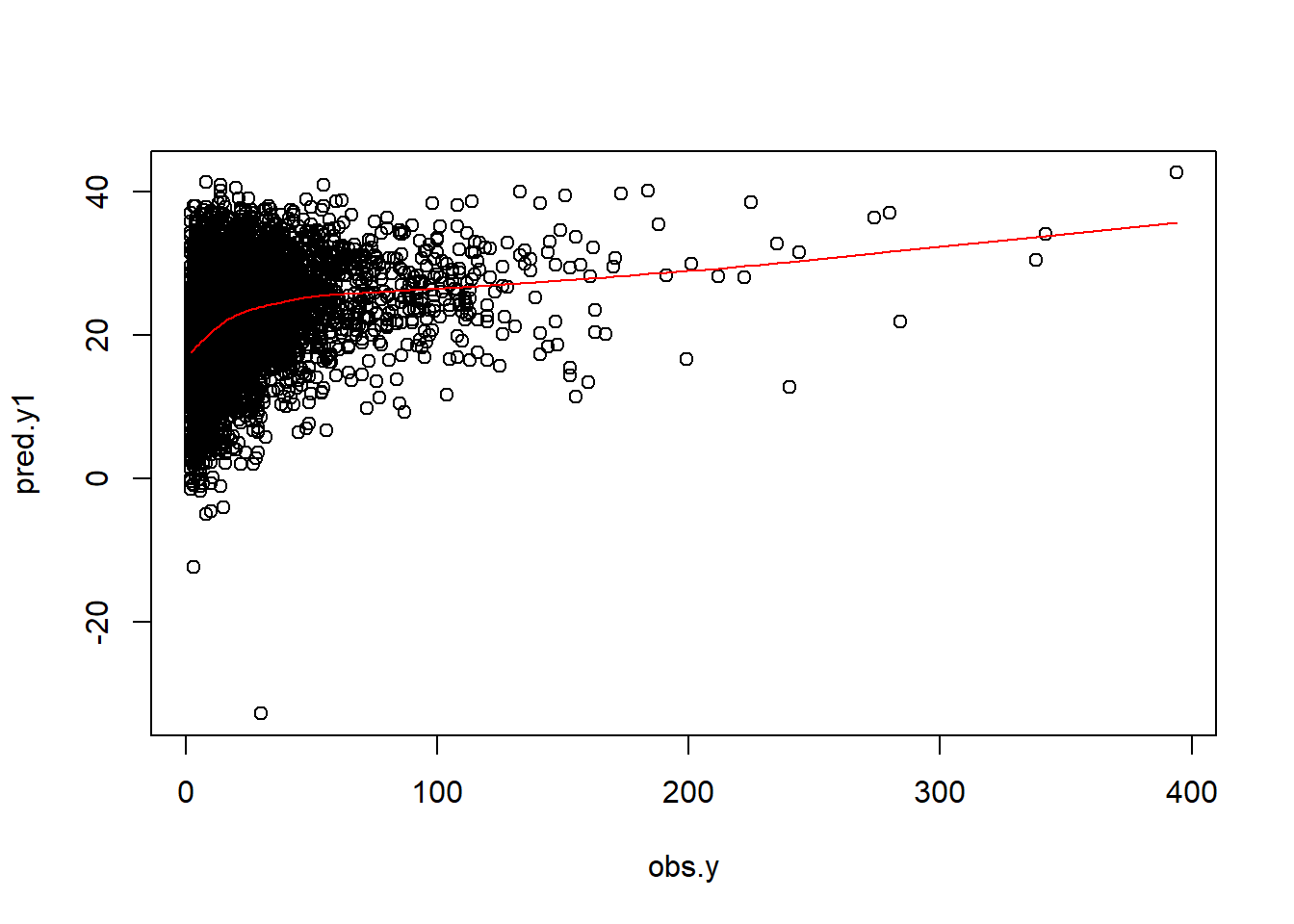
Measuring prediction error
Prediction error measures how well the model can predict the outcome for new data that were not used in developing the prediction model.
- Bias reduced for models with more variables
- Unimportant variables lead to noise / variability
- Bias variance trade-off / need penalization
R2
The provided information describes a statistical context involving a dataset of n values, \(y_1, ..., y_n\) (referred to as \(y_i\) or as a vector \(y = [y_1,...,y_n]^T\)), each paired with a fitted value \(f_1,...,f_n\) (denoted as \(f_i\) or sometimes \(\hat{y_i}\), and as a vector \(f\)). The residuals, represented as \(e_i\), are defined as the differences between the observed and the fitted values: $ e_i = y_i − f_i$
The mean of the observed data is denoted by \[ \bar{y} = \frac{1}{n}\sum_{i=1}^{n}y_i \]
The variability of the dataset can be quantified using two sums of squares formulas: 1. Residual Sum of Squares (SSres) or SSE: It quantifies the variance remaining in the data after fitting a model, calculated as: \[ SS_{res} = \sum_{i}(y_i - f_i)^2 = \sum_{i}e_i^2 \] 2. Total Sum of Squares (SStot) or SST: It represents the total variance in the observed data, calculated as: \[ SS_{tot} = \sum_{i}(y_i - \bar{y})^2 \]
The Coefficient of Determination (R²) or R.2, which provides a measure of how well the model’s predictions match the observed data, is defined as: \[ R^2 = 1 - \frac{SS_{res}}{SS_{tot}} \]
In the ideal scenario where the model fits the data perfectly, we have \(SS_{res} = 0\) and thus \(R^2 = 1\). Conversely, a baseline model, which always predicts the mean \(\bar{y}\) of the observed data, would yield \(R^2 = 0\). Models performing worse than this baseline model would result in a negative R² value. This metric is widely utilized in regression analysis to evaluate model performance, where a higher R² indicates a better fit of the model to the data.
RMSE
The root mean squared error (RMSE) uses the sample size \(n\) in the denominator, \(\sqrt{SS_{res}/n}\), and matches caret::RMSE. By contrast, \(\sqrt{SS_{res}/(n-p)}\) is the residual standard error (it divides by the residual degrees of freedom \(n-p\)), so the two quantities are not identical.
See (Wikipedia 2023b)
Adj R2
The Adjusted R² statistic modifies the \(R^2\) value to counteract the automatic increase of \(R^2\) when extra explanatory variables are added to a model, even if they do not improve the model fit. This adjustment is crucial for ensuring that the metric offers a reliable indication of the explanatory power of the model, especially in multiple regression where several predictors are involved.
The commonly used formula is defined as:
\[ \bar{R}^{2} = 1 - \frac{SS_{\text{res}} / df_{\text{res}}}{SS_{\text{tot}} / df_{\text{tot}}} \]
Where:
- \(SS_{\text{res}}\) and \(SS_{\text{tot}}\) represent the residual and total sums of squares respectively.
-
\(df_{\text{res}}\) and \(df_{\text{tot}}\) refer to the degrees of freedom of the residual and total sums of squares. Usually, \(df_{\text{res}} = n - p\) and \(df_{\text{tot}} = n - 1\), where:
- \(n\) signifies the sample size.
-
\(p\) denotes the number of parameters in the model, including the intercept (as defined above,
p <- dim(model.matrix(fit1))[2]).
This metric plays a vital role in model selection and safeguards against overfitting by penalizing the inclusion of non-informative variables
The alternate formula, written with an intercept-inclusive \(p\), is:
\[ \bar{R}^2 = 1 - (1 - R^2) \frac{n-1}{n-p} \]
This formula modifies the \(R^2\) value, accounting for the number of predictors and offering a more parsimonious model fit measure. Note that here \(p\) counts the intercept; in the more common textbook form \(\bar{R}^2 = 1 - (1 - R^2)\frac{n-1}{n-p-1}\), the symbol \(p\) denotes the number of predictors excluding the intercept, so the two expressions agree.
See (Wikipedia 2023a)
Overfitting and Optimism
- Model usually performs very well in the empirical data where the model was fitted in the same data (optimistic)
- Model performs poorly in the new data (generalization is not as good)
Causes
- Model determined by data at hand without expert opinion
- Too many model parameters (\(age\), \(age^2\), \(age^3\)) / predictors
- Too small dataset (training) / data too noisy
Consequences
- Overestimation of effects of predictors
- Reduction in model performance in new observations
Proposed solutions
We generally use procedures such as
- Internal validation
- sample splitting
- cross-validation
- bootstrap
- External validation
- Temporal
- Geographical
- Different data source to calculate same variable
- Different disease
Video content (optional)
Tip
For those who prefer a video walkthrough, feel free to watch the video below, which offers a description of an earlier version of the above content.
References
Wikipedia. 2023a. “Coefficient of Determination.” https://en.wikipedia.org/wiki/Coefficient_of_determination.
———. 2023b. “One-Way Analysis of Variance.” https://en.wikipedia.org/wiki/One-way_analysis_of_variance.