Simpson’s Paradox
Introduction
In this tutorial, we will use simcausal in R to simulate data and demonstrate how Simpson’s Paradox arises in a birthweight example similar to the “Birthweight Paradox” discussed by Hernández-Díaz et al. (2006). The paradox arises when adjusting for birthweight, leading to misleading conclusions about the relationship between maternal smoking and infant mortality. We will show how improper adjustment for birthweight, a collider in this context, can lead to biased estimates, and how to correct for this.
Birth Weight Paradox
Studies showed that while maternal smoking increased the risk of low birth weight (LBW) and infant mortality, among LBW infants, those born to smokers had lower infant mortality than LBW infants born to non-smokers. This seemingly paradoxical finding suggests that smoking could be “protective” for LBW infants, contradicting the established harmful effects of smoking during pregnancy.
This is a classic example of Simpson’s Paradox. The statistical reversal happens upon stratification, and the reason in this specific causal structure is that birthweight acts as a collider. Understanding this causal role is the only way to determine whether the stratified or unstratified result is the correct one for our research question.
Data Generation
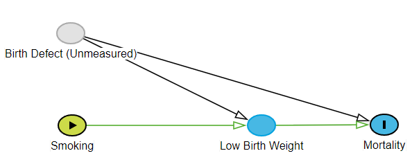
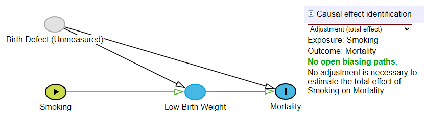
A Directed Acyclic Graph (DAG) is more than a mere illustration; it is a formal representation of a set of non-parametric causal assumptions about the data-generating process. The DAG provided in the tutorial encapsulates the hypothesized relationships between maternal smoking, an unmeasured factor, low birthweight, and infant mortality.
Setup
We will use the following R packages:
Data Generation
We will generate data to simulate the birthweight paradox. We assume that:
- Smoking influences Birthweight (low birth weight).
- Birthweight influences Infant Mortality.
- There are unmeasured factors (e.g., birth defects) that also influence both birthweight and infant mortality.
We will set up this data generating process using simcausal.
D <- DAG.empty()
D <- D +
  node("Smoking", distr = "rbern", prob = 0.3) +
  node("Unmeasured", distr = "rbern", prob = 0.2) +
  node("LowBirthweight", distr = "rbern", prob = plogis(-1 + 1.5*Smoking + 2*Unmeasured)) +
  node("Mortality", distr = "rbern", prob = plogis(-2 + 4*LowBirthweight + 4*Unmeasured))

Dset <- set.DAG(D)
Visualizing the DAG
Let’s plot the DAG to see how these variables are related:
plotDAG(Dset, xjitter = 0.1, yjitter = 0.1,
        edge_attrs = list(width = 1, arrow.width = 1, arrow.size = 1),
        vertex_attrs = list(size = 15, label.cex = 0.8))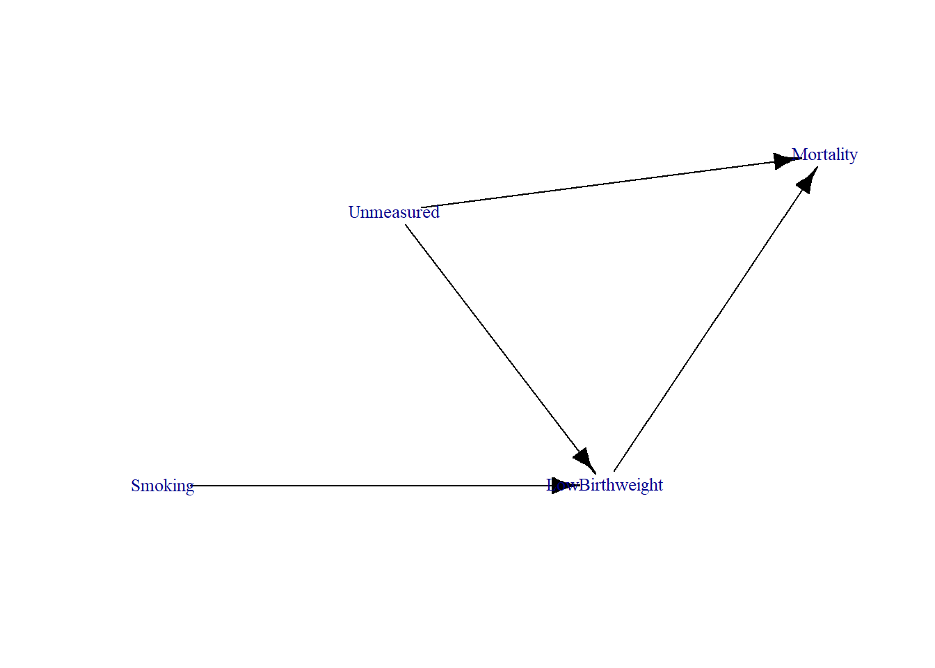
This DAG represents the relationships between maternal smoking, low birth weight, and mortality, with an unmeasured confounder affecting both birthweight and mortality. Low birth weight is a collider because it has two incoming arrows from both Smoking and Birth Defect (Unmeasured).
The Dual Role of Low Birthweight: Mediator and Collider
The key to this puzzle is that LowBirthweight plays two different and conflicting roles depending on which causal path you examine.
Mediator: On the path Smoking → LowBirthweight → Mortality, LBW is a mediator. It is a mechanism through which smoking causes death. Smoking leads to LBW, which in turn leads to mortality. The purpose of mediation analysis is often to isolate the direct effect from this indirect, mediated path.
Collider: On the path Smoking → LowBirthweight ← Unmeasured, LBW is a collider. A collider is a variable that is a common effect of two other variables (arrows “collide” into it). The fundamental rule of DAGs concerning colliders is that one must not condition on them or their descendants. Conditioning on a collider opens the non-causal path between its parents, inducing a spurious statistical association where none may have existed before. Conditioning on a collider (by adjusting for it in a model or stratifying by it) is a major analytical error.
This dual role creates an analytical trap. The statistical act of adjusting for LowBirthweight—which you might do to block its mediating effect—simultaneously conditions on it as a collider. This opens a spurious “backdoor” path between Smoking and the Unmeasured factors, introducing severe bias and leading to the paradoxical conclusion.
Simulate Data
We now simulate data based on the DAG structure.
sim_data <- sim(Dset, n = 10000, rndseed = 123)
#> simulating observed dataset from the DAG object
head(sim_data) %>%
  kable("html", caption = "First 6 Rows of Simulated Data") %>%
  kable_styling(bootstrap_options = c("striped", "hover", "condensed", "responsive"),
                full_width = FALSE,
position = "center")| ID | Smoking | Unmeasured | LowBirthweight | Mortality |
|---|---|---|---|---|
| 1 | 0 | 0 | 1 | 1 |
| 2 | 1 | 0 | 1 | 1 |
| 3 | 0 | 1 | 1 | 1 |
| 4 | 1 | 0 | 1 | 1 |
| 5 | 1 | 0 | 0 | 0 |
| 6 | 0 | 0 | 0 | 0 |
Visualizing Hypothetical Distributions
# Simulate continuous birth weight based on binary LowBirthweight variable
set.seed(123)
sim_data$BirthWeight <- ifelse(sim_data$LowBirthweight == 1,
                               rnorm(n = sum(sim_data$LowBirthweight == 1),
                                     mean = 2200, sd = 300),  # Low birthweight
                               rnorm(n = sum(sim_data$LowBirthweight == 0),
                                     mean = 3300, sd = 500))  # Normal birthweight
sim_data$Smoking <- factor(sim_data$Smoking,
                           levels = c(0, 1),
                           labels = c("Non-smoking", "Smoking"))
sim_data$LowBirthweight <- factor(sim_data$LowBirthweight,
                                  levels = c(0, 1),
                                  labels = c("Normal Birthweight", "Low Birthweight"))
# Create a density plot for birth weight distribution by smoking status
ggplot(sim_data, aes(x = BirthWeight, fill = Smoking, color = Smoking)) +
  geom_density(alpha = 0.3, size = 1.2) +
  geom_vline(xintercept = 2500, linetype = "solid", color = "black", size = 1) +
  scale_fill_manual(values = c("Smoking" = "red", "Non-smoking" = "blue")) +
  scale_color_manual(values = c("Smoking" = "red", "Non-smoking" = "blue")) +
  labs(title = "Distribution of Birth Weights by Smoking Status",
    subtitle = "Low Birth Weight (LBW) is typically defined as a birth weight of less than 2,500 grams",
       x = "Birth Weight (g)",
       y = "Density",
       fill = "Smoking Status",
       color = "Smoking Status") +
  theme_minimal() +
  theme(legend.position = "top")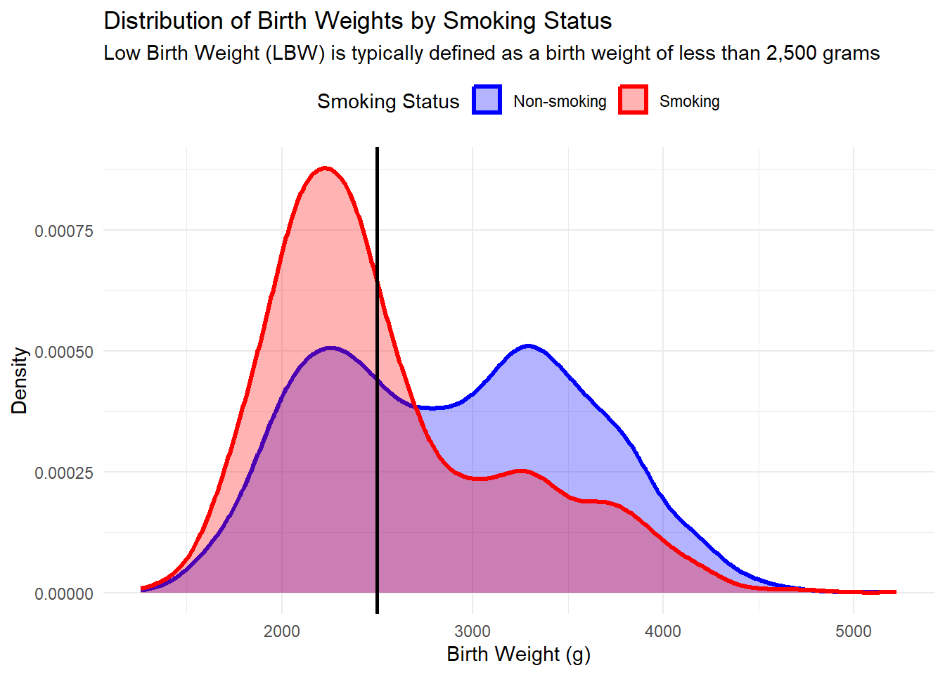
Analysis
Crude Bivariate Relationships
# Calculate the summary statistics (mean birth weight, LBW prevalence, and mortality prevalence) by smoking status
summary_stats <- sim_data %>%
  group_by(Smoking) %>%
  summarise(
    mean_birthweight = mean(BirthWeight, na.rm = TRUE),  # Mean birth weight
    prevalence_LBW = mean(LowBirthweight == "Low Birthweight") * 100,  # Prevalence of LBW in percentage
    prevalence_mortality = mean(Mortality) * 100  # Prevalence of mortality in percentage
  ) %>%
  mutate(
    mean_birthweight = format(round(mean_birthweight, 1), big.mark = ","),  # Round and format birth weight
    prevalence_LBW = round(prevalence_LBW, 1),  # Round LBW prevalence to 1 decimal place
    prevalence_mortality = round(prevalence_mortality, 1)  # Round mortality prevalence to 1 decimal place
  )

# Display the formatted table with kable
summary_stats %>%
  kable("html", caption = "Summary Statistics: Mean Birth Weight, LowBirthWeight (LBW) Prevalence, and Mortality Prevalence") %>%
  kable_styling(bootstrap_options = c("striped", "hover", "condensed", "responsive"),
                full_width = FALSE,
position = "center")| Smoking | mean_birthweight | prevalence_LBW | prevalence_mortality |
|---|---|---|---|
| Non-smoking | 2,895.1 | 36.6 | 45.8 |
| Smoking | 2,552.5 | 67.9 | 66.2 |
Analysis Part 1: Attempting to Estimate the Direct Effect
We now show what happens when we adjust for LowBirthweight, which acts as a collider.
# Model adjusted for LowBirthweight (incorrect adjustment)
fit_incorrect <- glm(Mortality ~ Smoking + LowBirthweight, family = binomial(), data = sim_data)
publish(fit_incorrect, print = FALSE)$regressionTable %>%
  kable("html", caption = "Adjusted Model Regression Table") %>%
  kable_styling(bootstrap_options = c("striped", "hover", "condensed", "responsive"),
                full_width = FALSE,
position = "center")| Variable | Units | OddsRatio | CI.95 | p-value |
|---|---|---|---|---|
| Smoking | Non-smoking | Ref | ||
| Smoking | 0.73 | [0.63;0.84] | <1e-04 | |
| LowBirthweight | Normal Birthweight | Ref | ||
| Low Birthweight | 59.40 | [51.75;68.18] | <1e-04 |
Explanation: To estimate the direct effect of smoking (the effect not mediated through birthweight), the standard approach would be to adjust for the mediator, LowBirthweight. However, in this causal structure, this adjustment is incorrect because it simultaneously conditions on a collider. This opens a spurious backdoor path between Smoking and Unmeasured, introducing collider bias. The resulting odds ratio of 0.73 is not a valid estimate of the direct effect; it is a hopelessly biased number.
Stratification
We will now stratify the data by Low Birthweight and calculate the effect of smoking on mortality separately for low birthweight and normal birthweight infants.
# Subset for low birthweight
fit_stratified_LBW <- glm(Mortality ~ Smoking, family = binomial(), data = subset(sim_data, LowBirthweight == "Low Birthweight"))
publish(fit_stratified_LBW, print = FALSE)$regressionTable %>%
  kable("html", caption = "Stratified Model Regression Table") %>%
  kable_styling(bootstrap_options = c("striped", "hover", "condensed", "responsive"),
                full_width = FALSE,
position = "center")| Variable | Units | OddsRatio | CI.95 | p-value |
|---|---|---|---|---|
| Smoking | Non-smoking | Ref | ||
| Smoking | 0.69 | [0.55;0.85] | 0.000565 |
# Subset for normal birthweight
fit_stratified_NBW <- glm(Mortality ~ Smoking, family = binomial(), data = subset(sim_data, LowBirthweight == "Normal Birthweight"))
publish(fit_stratified_NBW, print = FALSE)$regressionTable %>%
  kable("html", caption = "Stratified Model Regression Table") %>%
  kable_styling(bootstrap_options = c("striped", "hover", "condensed", "responsive"),
                full_width = FALSE,
position = "center")| Variable | Units | OddsRatio | CI.95 | p-value |
|---|---|---|---|---|
| Smoking | Non-smoking | Ref | ||
| Smoking | 0.77 | [0.63;0.93] | 0.007758 |
Interaction Approach
We include an interaction term between Smoking and LowBirthweight to test whether the effect of smoking on mortality differs by birthweight status.
fit_interaction <- glm(Mortality ~ Smoking * LowBirthweight, family = binomial(), data = sim_data)
publish(fit_interaction, print = FALSE)$regressionTable %>%
  kable("html", caption = "Interaction Model Regression Table") %>%
  kable_styling(bootstrap_options = c("striped", "hover", "condensed", "responsive"),
                full_width = FALSE,
position = "center")| Variable | Units | OddsRatio | CI.95 | p-value |
|---|---|---|---|---|
| Smoking(Non-smoking): LowBirthweight(Low Birthweight vs Normal Birthweight) | 61.73 | [52.00;73.28] | < 1e-04 | |
| Smoking(Smoking): LowBirthweight(Low Birthweight vs Normal Birthweight) | 55.21 | [43.70;69.74] | < 1e-04 | |
| LowBirthweight(Normal Birthweight): Smoking(Smoking vs Non-smoking) | 0.77 | [0.63;0.93] | 0.007758 | |
| LowBirthweight(Low Birthweight): Smoking(Smoking vs Non-smoking) | 0.69 | [0.55;0.85] | 0.000565 |
Correct Approach: No Adjustment for LowBirthweight
To estimate the total causal effect of smoking on mortality (the net effect through all pathways), we must not adjust for the mediator, LowBirthweight. Our DAG shows no other open backdoor paths that need blocking. Therefore, the unadjusted model correctly estimates the total causal effect.
# Correct model (no adjustment for LowBirthweight)
fit_correct <- glm(Mortality ~ Smoking, family = binomial(), data = sim_data)
publish(fit_correct, print = FALSE)$regressionTable %>%
  kable("html", caption = "Unadjusted Model Regression Table") %>%
  kable_styling(bootstrap_options = c("striped", "hover", "condensed", "responsive"),
                full_width = FALSE,
position = "center")| Variable | Units | OddsRatio | CI.95 | p-value |
|---|---|---|---|---|
| Smoking | Non-smoking | Ref | ||
| Smoking | 2.31 | [2.12;2.53] | <1e-04 |
Comparing Estimates
# Extract ORs from publish output for each model
or_incorrect <- publish(fit_incorrect, print = FALSE)$regressionTable[2, "OddsRatio"]
or_stratified_LBW <- publish(fit_stratified_LBW, print = FALSE)$regressionTable[2, "OddsRatio"]
or_stratified_NBW <- publish(fit_stratified_NBW, print = FALSE)$regressionTable[2, "OddsRatio"]
or_interaction1 <- publish(fit_interaction, print = FALSE)$regressionTable[3, "OddsRatio"]
or_interaction2 <- publish(fit_interaction, print = FALSE)$regressionTable[4, "OddsRatio"]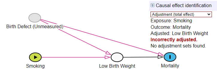
Now we compare the estimates from:
- The incorrect model (adjusted for LowBirthweight), with an OR of 0.73.
- The stratified model
- for low birthweight infants, with an OR of 0.69.
- for normal birthweight infants, with an OR of 0.77.
- The interaction model, where the OR for smokers is
- 0.69 (Low Birthweight),
- 0.77 (Normal Birthweight).
- The correct model (unadjusted for LowBirthweight), with an OR of 2.31.
These comparisons highlight how adjusting for a collider (Low Birthweight) introduces bias, while avoiding this adjustment gives an unbiased estimate of the effect of Smoking on Mortality.
Visualizing Estimates
# Helper function to clean and convert ORs and CIs
extract_or_ci <- function(or_str, ci_str) {
  or_val <- ifelse(or_str == "Ref", NA, as.numeric(or_str))  # Convert OR to numeric, handle Ref

  # Split the CI string, handle empty or malformed CI strings
  if (ci_str != "" && grepl("\\[", ci_str)) {
    ci_vals <- as.numeric(gsub("\\[|\\]", "", unlist(strsplit(ci_str, ";"))))  # Split and convert CI
  } else {
    ci_vals <- c(NA, NA)  # Handle missing CIs
  }

  return(list(OR = or_val, CI.lower = ci_vals[1], CI.upper = ci_vals[2]))
}

# Extract ORs and CIs for each model using the helper function
or_ci_incorrect <- extract_or_ci(publish(fit_incorrect, print = FALSE)$regressionTable[2, "OddsRatio"],
                                 publish(fit_incorrect, print = FALSE)$regressionTable[2, "CI.95"])

or_ci_stratified_LBW <- extract_or_ci(publish(fit_stratified_LBW, print = FALSE)$regressionTable[2, "OddsRatio"],
                                      publish(fit_stratified_LBW, print = FALSE)$regressionTable[2, "CI.95"])

or_ci_stratified_NBW <- extract_or_ci(publish(fit_stratified_NBW, print = FALSE)$regressionTable[2, "OddsRatio"],
                                      publish(fit_stratified_NBW, print = FALSE)$regressionTable[2, "CI.95"])

or_ci_interaction1 <- extract_or_ci(publish(fit_interaction, print = FALSE)$regressionTable[3, "OddsRatio"],
                                    publish(fit_interaction, print = FALSE)$regressionTable[3, "CI.95"])

or_ci_interaction2 <- extract_or_ci(publish(fit_interaction, print = FALSE)$regressionTable[4, "OddsRatio"],
                                    publish(fit_interaction, print = FALSE)$regressionTable[4, "CI.95"])

or_ci_correct <- extract_or_ci(publish(fit_correct, print = FALSE)$regressionTable[2, "OddsRatio"],
                               publish(fit_correct, print = FALSE)$regressionTable[2, "CI.95"])
# Step 2: Create a data frame for the forest plot
forest_data <- data.frame(
Model = c("Incorrect (Adjusted for LBW)",
"Stratified (Low Birthweight)",
"Stratified (Normal Birthweight)",
"Interaction (Low Birthweight)",
"Interaction (Normal Birthweight)",
"Correct (Unadjusted)"),
OR = c(or_ci_incorrect$OR, or_ci_stratified_LBW$OR, or_ci_stratified_NBW$OR, or_ci_interaction2$OR, or_ci_interaction1$OR, or_ci_correct$OR),
CI.lower = c(or_ci_incorrect$CI.lower, or_ci_stratified_LBW$CI.lower, or_ci_stratified_NBW$CI.lower, or_ci_interaction2$CI.lower, or_ci_interaction1$CI.lower, or_ci_correct$CI.lower),
CI.upper = c(or_ci_incorrect$CI.upper, or_ci_stratified_LBW$CI.upper, or_ci_stratified_NBW$CI.upper, or_ci_interaction2$CI.upper, or_ci_interaction1$CI.upper, or_ci_correct$CI.upper)
)
# Display the data frame to ensure it's correct
print(forest_data)
#> Model OR CI.lower CI.upper
#> 1 Incorrect (Adjusted for LBW) 0.73 0.63 0.84
#> 2 Stratified (Low Birthweight) 0.69 0.55 0.85
#> 3 Stratified (Normal Birthweight) 0.77 0.63 0.93
#> 4 Interaction (Low Birthweight) 0.69 0.55 0.85
#> 5 Interaction (Normal Birthweight) 0.77 0.63 0.93
#> 6 Correct (Unadjusted) 2.31 2.12 2.53# Create the forest plot
ggplot(forest_data, aes(x = OR, y = Model)) +
geom_point(size = 3) +
geom_errorbarh(aes(xmin = CI.lower, xmax = CI.upper), height = 0.2) +
geom_vline(xintercept = 1, linetype = "dashed", color = "red") + # Reference line at OR = 1
labs(title = "Forest Plot of OR",
x = "Odds Ratio (OR) and Confidence Intervals",
y = "") +
theme_minimal() +
theme(axis.text.y = element_text(size = 12),
axis.title.x = element_text(size = 14),
plot.title = element_text(size = 16, face = "bold"))
#> Warning: `geom_errorbarh()` was deprecated in ggplot2 4.0.0.
#> ℹ Please use the `orientation` argument of `geom_errorbar()` instead.
#> `height` was translated to `width`.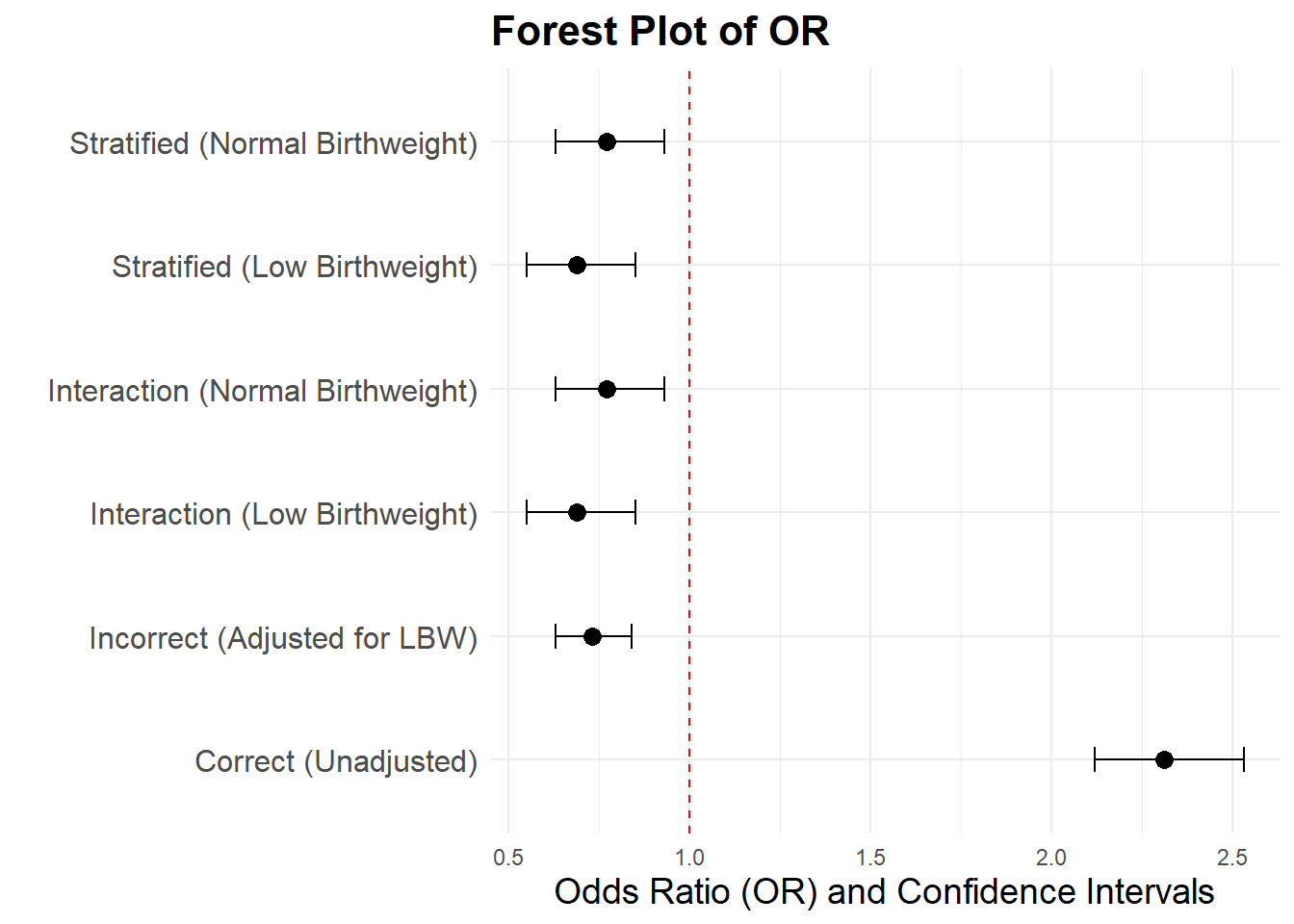
Clarifying the Target: Total Effect vs. Direct Effect
A frequent source of confusion in causal analysis is the failure to distinguish between different causal questions, or “estimands.” The tutorial correctly demonstrates how to estimate the total causal effect of smoking, while the user’s query focuses on the direct effect. These are distinct quantities that require different analytical strategies.
Total Effect (TE): This estimand represents the overall impact of the exposure on the outcome, encompassing all causal pathways. It answers the question: “What is the net effect of a mother smoking versus not smoking on the risk of infant mortality?” To estimate the TE, an analyst must block all non-causal “back-door” paths between the exposure and outcome. In the provided DAG, there are no open back-door paths from
SmokingtoMortality. The path throughLowBirthweightis a front-door (causal) path, and the path involving theUnmeasuredvariable is blocked by the colliderLowBirthweight. Therefore, as the tutorial’s “Correct Approach” shows, the total causal effect is correctly estimated by a simple unadjusted regression ofMortalityonSmoking, which yields an Odds Ratio (OR) of 2.31.Direct Effect: This estimand represents the effect of the exposure on the outcome that does not operate through a specific mediator. It answers the question: “What is the effect of a mother smoking on infant mortality, independent of its effect on the baby’s birth weight?” As noted above, the conventional (though in this case, incorrect) approach to isolating this effect is to include the mediator as a covariate in a regression model. The tutorial’s “Incorrect Adjustment” section performs exactly this, regressing
Mortalityon bothSmokingandLowBirthweight.
Causal Questions Dictate Correct Methods
The Birthweight Paradox is a powerful lesson in causal inference. It demonstrates that a naive statistical adjustment, without regard for the underlying causal structure, can produce results that are not just wrong, but dangerously misleading.
The “paradox” is resolved by causal reasoning: The reversal is caused by conditioning on
LowBirthweight, a variable that is simultaneously a mediator of the effect we want to study and a collider that introduces bias from an unmeasured variable.-
The analysis must match the question:
To estimate the total effect of smoking, we must not adjust for the mediator/collider. The unadjusted OR of 2.31 is the correct estimate for this question.
Estimating the direct effect is not possible with simple adjustment in this scenario. The adjusted OR of 0.73 is a biased artifact and does not represent a real causal effect.
Estimating the direct effect (“What is the effect of smoking on mortality that is not mediated by birthweight?”) is “not possible with simple adjustment” because the necessary information to disentangle the direct effect from the confounding effect of the Unmeasured variable is simply not present in the observable data (Smoking, LowBirthweight, Mortality). No matter how sophisticated a regression model one fits using only these observed variables, it cannot recover an unbiased estimate of the (natural) direct effect. The problem is not with the statistical tool, but with the fundamental limits of what the data can reveal given the causal reality depicted by the DAG. The language of potential outcomes makes this challenge explicit, as it requires estimating “cross-world” counterfactuals (e.g., the outcome under smoking with the mediator at its non-smoking level), which is impossible when an unmeasured confounder links the worlds of the mediator and the outcome.
Advanced methods such as instrumental variable analysis represents a powerful theoretical alternative for achieving identification in the face of unmeasured confounding. However, it should not be seen as a simple or universally applicable solution. It requires a fundamental shift in the “burden of belief” from the assumption of no unmeasured confounding (sequential ignorability) to a different, and often more stringent, set of untestable assumptions about the existence of a valid instrument. The choice between these analytical frameworks is not a statistical one, but a scientific one, based on which set of assumptions is most defensible in a specific research context.
- Key Insight: The most important step in an analysis is to draw a DAG based on subject-matter knowledge. This causal map is essential for identifying which variables to adjust for and which to leave alone to answer your specific research question correctly.