Overfitting and performance

The following tutorial extends the work from the previous lab and focuses on understanding overfitting, evaluating performance, and function writing in the context of linear modeling for a continuous outcome variable, cholesterol levels.

# Load required packages
library(caret)
library(knitr)
library(Publish)
library(car)

Load data

Load the data saved at the end of previous part of the lab.

load(file="Data/predictivefactors/cholesterolNHANES15part2.RData")

Now we will fit the final model that we decided at the end of previous part of the lab.

formula4 <- as.formula("cholesterol~gender + age + born + 
             race + education + married + 
             income + diastolicBP + systolicBP + 
             bmi + triglycerides + uric.acid + 
             protein + bilirubin + phosphorus + sodium + potassium + 
             globulin + calcium + physical.work + 
             physical.recreational + diabetes")
formula4
#> cholesterol ~ gender + age + born + race + education + married + 
#>     income + diastolicBP + systolicBP + bmi + triglycerides + 
#>     uric.acid + protein + bilirubin + phosphorus + sodium + potassium + 
#>     globulin + calcium + physical.work + physical.recreational + 
#>     diabetes
fit4 <- lm(formula4, data = analytic3)
summary(fit4)
#> 
#> Call:
#> lm(formula = formula4, data = analytic3)
#> 
#> Residuals:
#>      Min       1Q   Median       3Q      Max 
#> -115.465  -23.695   -2.598   20.017  177.264 
#> 
#> Coefficients:
#>                             Estimate Std. Error t value Pr(>|t|)    
#> (Intercept)               136.871606  51.998527   2.632  0.00853 ** 
#> genderMale                -13.064857   1.802099  -7.250 5.48e-13 ***
#> age                         0.351838   0.056116   6.270 4.22e-10 ***
#> bornOthers                  7.877420   1.947498   4.045 5.39e-05 ***
#> raceHispanic               -5.790547   2.323010  -2.493  0.01274 *  
#> raceOther                  -4.879882   2.781673  -1.754  0.07950 .  
#> raceWhite                  -0.847635   2.130149  -0.398  0.69072    
#> educationHigh.School        2.851633   1.617435   1.763  0.07801 .  
#> educationSchool            -2.446765   3.084409  -0.793  0.42769    
#> marriedNever.married       -5.739509   1.997152  -2.874  0.00409 ** 
#> marriedPreviously.married   0.342206   1.968165   0.174  0.86198    
#> incomeBetween.25kto54k     -0.867063   1.990253  -0.436  0.66312    
#> incomeBetween.55kto99k      2.462130   2.169757   1.135  0.25658    
#> incomeOver100k              2.626046   2.394560   1.097  0.27289    
#> diastolicBP                 0.374971   0.062238   6.025 1.93e-09 ***
#> systolicBP                  0.029976   0.049515   0.605  0.54497    
#> bmi                        -0.309530   0.118927  -2.603  0.00930 ** 
#> triglycerides               0.124806   0.006427  19.419  < 2e-16 ***
#> uric.acid                   1.357242   0.609012   2.229  0.02593 *  
#> protein                     4.767008   2.931636   1.626  0.10406    
#> bilirubin                  -6.060791   2.593508  -2.337  0.01952 *  
#> phosphorus                 -0.076472   1.341957  -0.057  0.95456    
#> sodium                     -1.026686   0.347679  -2.953  0.00318 ** 
#> potassium                   0.893507   2.283488   0.391  0.69561    
#> globulin                   -2.198037   3.036091  -0.724  0.46915    
#> calcium                    12.202366   2.574400   4.740 2.25e-06 ***
#> physical.workYes           -0.439108   1.651078  -0.266  0.79030    
#> physical.recreationalYes    1.238756   1.667670   0.743  0.45767    
#> diabetesYes               -19.032748   2.158825  -8.816  < 2e-16 ***
#> ---
#> Signif. codes:  0 '***' 0.001 '**' 0.01 '*' 0.05 '.' 0.1 ' ' 1
#> 
#> Residual standard error: 35.22 on 2603 degrees of freedom
#> Multiple R-squared:  0.2415, Adjusted R-squared:  0.2334 
#> F-statistic: 29.61 on 28 and 2603 DF,  p-value: < 2.2e-16

Design Matrix

Expands factors to a set of dummy variables.

Tip

We can use the model.matrix function to construct a design/model matrix, such as expand factor variables to a matrix of dummy variable

The dimensions of the model matrix are obtained, and the total number of model parameters (p) is calculated.

head(model.matrix(fit4))
#>    (Intercept) genderMale age bornOthers raceHispanic raceOther raceWhite
#> 1            1          1  62          0            0         0         1
#> 2            1          1  53          1            0         0         1
#> 4            1          0  56          0            0         0         1
#> 5            1          0  42          0            0         0         0
#> 10           1          1  22          0            0         0         0
#> 11           1          0  32          1            1         0         0
#>    educationHigh.School educationSchool marriedNever.married
#> 1                     0               0                    0
#> 2                     1               0                    0
#> 4                     0               0                    0
#> 5                     0               0                    0
#> 10                    0               0                    1
#> 11                    0               0                    0
#>    marriedPreviously.married incomeBetween.25kto54k incomeBetween.55kto99k
#> 1                          0                      0                      1
#> 2                          1                      0                      0
#> 4                          0                      0                      1
#> 5                          1                      1                      0
#> 10                         0                      1                      0
#> 11                         0                      1                      0
#>    incomeOver100k diastolicBP systolicBP  bmi triglycerides uric.acid protein
#> 1               0          70        128 27.8           158       4.2     7.5
#> 2               0          88        146 30.8           170       7.0     7.4
#> 4               0          72        132 42.4            93       5.4     6.1
#> 5               0          70        100 20.3            52       3.3     7.7
#> 10              0          70        110 28.0            77       6.0     7.4
#> 11              0          70        120 28.2           295       5.2     7.4
#>    bilirubin phosphorus sodium potassium globulin calcium physical.workYes
#> 1        0.5        4.7    136      4.30      2.9     9.8                0
#> 2        0.6        4.4    140      4.55      2.9     9.8                0
#> 4        0.3        3.8    141      4.08      2.3     8.9                0
#> 5        0.3        3.2    136      3.50      3.4     9.3                0
#> 10       0.2        5.3    139      4.16      3.0     9.3                0
#> 11       0.4        3.1    138      4.31      2.9    10.3                0
#>    physical.recreationalYes diabetesYes
#> 1                         0           1
#> 2                         0           0
#> 4                         0           0
#> 5                         0           0
#> 10                        1           0
#> 11                        0           0

# Dimension of the model matrix
dim(model.matrix(fit4))
#> [1] 2632   29

# Number of parameters = intercept + slopes
p <- dim(model.matrix(fit4))[2] 
p
#> [1] 29

Check prediction

The observed and predicted cholesterol values are summarized.

obs.y <- analytic3$cholesterol
summary(obs.y)
#>    Min. 1st Qu.  Median    Mean 3rd Qu.    Max. 
#>    81.0   163.0   189.0   191.5   216.0   362.0

# Predict the above fit on analytic3 data
pred.y <- predict(fit4, analytic3)
summary(pred.y)
#>    Min. 1st Qu.  Median    Mean 3rd Qu.    Max. 
#>   136.3   178.2   189.4   191.5   202.4   337.6
n <- length(pred.y)
n
#> [1] 2632
plot(obs.y,pred.y)
lines(lowess(obs.y,pred.y), col = "red")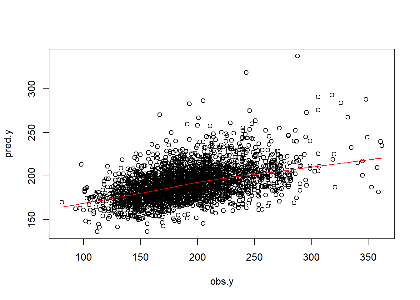

# Prediction on a new data: fictitious.data
str(fictitious.data)
#> 'data.frame':    4121 obs. of  33 variables:
#>  $ ID                   : num  83732 83733 83734 83735 83736 ...
#>  $ gender               : chr  "Male" "Male" "Male" "Female" ...
#>  $ age                  : num  62 53 78 56 42 72 22 32 56 46 ...
#>  $ born                 : chr  "Born in 50 US states or Washingt" "Others" "Born in 50 US states or Washingt" "Born in 50 US states or Washingt" ...
#>  $ race                 : chr  "White" "White" "White" "White" ...
#>  $ education            : chr  "College" "High.School" "High.School" "College" ...
#>  $ married              : chr  "Married" "Previously.married" "Married" "Married" ...
#>  $ income               : chr  "Between.55kto99k" "<25k" "<25k" "Between.55kto99k" ...
#>  $ weight               : num  135630 25282 12576 102079 18235 ...
#>  $ psu                  : num  1 1 1 1 2 1 2 1 2 1 ...
#>  $ strata               : num  125 125 131 131 126 128 128 125 126 121 ...
#>  $ diastolicBP          : num  70 88 46 72 70 58 70 70 116 94 ...
#>  $ systolicBP           : num  128 146 138 132 100 116 110 120 178 144 ...
#>  $ bodyweight           : num  94.8 90.4 83.4 109.8 55.2 ...
#>  $ bodyheight           : num  184 171 170 161 165 ...
#>  $ bmi                  : num  27.8 30.8 28.8 42.4 20.3 28.6 28 28.2 33.6 27.6 ...
#>  $ waist                : num  101.1 107.9 116.5 110.1 80.4 ...
#>  $ smoke                : chr  "Not.at.all" "Every.day" "Not.at.all" "Not.at.all" ...
#>  $ alcohol              : num  1 6 0 1 1 0 8 1 0 1 ...
#>  $ cholesterol          : num  173 265 229 174 204 190 164 190 145 242 ...
#>  $ cholesterolM2        : num  4.47 6.85 5.92 4.5 5.28 4.91 4.24 4.91 3.75 6.26 ...
#>  $ triglycerides        : num  158 170 299 93 52 52 77 295 121 497 ...
#>  $ uric.acid            : num  4.2 7 7.3 5.4 3.3 4.9 6 5.2 4.8 6.5 ...
#>  $ protein              : num  7.5 7.4 7.3 6.1 7.7 7.1 7.4 7.4 6.9 6.8 ...
#>  $ bilirubin            : num  0.5 0.6 0.5 0.3 0.3 0.5 0.2 0.4 0.4 0.5 ...
#>  $ phosphorus           : num  4.7 4.4 3.6 3.8 3.2 3.7 5.3 3.1 4.1 3.6 ...
#>  $ sodium               : num  136 140 140 141 136 140 139 138 140 138 ...
#>  $ potassium            : num  4.3 4.55 4.7 4.08 3.5 4.2 4.16 4.31 4.5 4.27 ...
#>  $ globulin             : num  2.9 2.9 2.8 2.3 3.4 3 3 2.9 2.9 2.6 ...
#>  $ calcium              : num  9.8 9.8 9.7 8.9 9.3 9.3 9.3 10.3 9.5 9.3 ...
#>  $ physical.work        : chr  "No" "No" "No" "No" ...
#>  $ physical.recreational: chr  "No" "No" "No" "No" ...
#>  $ diabetes             : chr  "Yes" "No" "Yes" "No" ...
#>  - attr(*, "na.action")= 'omit' Named int [1:885] 16 30 39 48 50 58 61 65 67 68 ...
#>   ..- attr(*, "names")= chr [1:885] "27" "68" "90" "112" ...
pred.y.new1 <- predict(fit4, fictitious.data)
summary(pred.y.new1)
#>    Min. 1st Qu.  Median    Mean 3rd Qu.    Max. 
#>   128.7   178.9   190.6   192.5   203.3   557.4

Measuring prediction error

Continuous outcomes

R2

The Sum of Squares of Errors (SSE) and the Total Sum of Squares (SST) are calculated. The proportion of variance explained by the model is then calculated as R2.

See Wikipedia (2023a)

# Find SSE
SSE <- sum( (obs.y - pred.y)^2 )
SSE
#> [1] 3228460

# Find SST
mean.obs.y <- mean(obs.y)
SST <- sum( (obs.y - mean.obs.y)^2 )
SST
#> [1] 4256586

# Find R2
R.2 <- 1- SSE/SST
R.2
#> [1] 0.2415378

require(caret)
R2(pred.y, obs.y)
#> [1] 0.2415378

RMSE

The Root Mean Square Error is calculated to measure the average magnitude of the errors between predicted and observed values.

See Wikipedia (2023b)

# Find RMSE
Rmse <- sqrt(SSE/(n-p)) 
Rmse
#> [1] 35.21767

RMSE(pred.y, obs.y)
#> [1] 35.02311

Adj R2

It provides a measure of how well the model generalizes and adjusts R2 based on the number of predictors.

See Wikipedia (2023a)

# Find adj R2
adjR2 <- 1-(1-R.2)*((n-1)/(n-p))
adjR2
#> [1] 0.2333791

Writing function

Syntax for Writing Functions

func_name <- function (argument) {
  A statement or multiple lines of statements
  return(output)
}

Example of a simple function

f1 <- function(a,b){
  result <- a + b
  return(result)
}
f1(a=1,b=3)
#> [1] 4
f1(a=1,b=6)
#> [1] 7
# setting default values
f1 <- function(a=1,b=1){
  result <- a + b
  return(result)
}
f1()
#> [1] 2
f1(b = 10)
#> [1] 11

A bit more complicated

# one argument
model.fit <- function(data.for.fitting){
  formulax <- as.formula("cholesterol~gender + age + born")
  fitx <- lm(formulax, data = data.for.fitting)
  result <- coef(fitx)
  return(result)
}
model.fit(data.for.fitting=analytic)
#> (Intercept)  genderMale         age  bornOthers 
#> 184.3131838  -7.8095595   0.2225745  11.1557140
model.fit(data.for.fitting=analytic3)
#> (Intercept)  genderMale         age  bornOthers 
#> 176.1286576  -4.8256829   0.3375009   7.7186190

# adding one more argument: digits
model.fit <- function(data.for.fitting, digits=2){
  formulax <- as.formula("cholesterol~gender + age + born")
  fitx <- lm(formulax, data = data.for.fitting)
  result <- coef(fitx)
  result <- round(result,digits)
  return(result)
}
model.fit(data.for.fitting=analytic)
#> (Intercept)  genderMale         age  bornOthers 
#>      184.31       -7.81        0.22       11.16
model.fit(data.for.fitting=analytic3)
#> (Intercept)  genderMale         age  bornOthers 
#>      176.13       -4.83        0.34        7.72

Function that gives performance measures

let us create a function that will give us the performance measures:

perform <- function(new.data,
                    model.fit,model.formula=NULL, 
                    y.name = "Y",
                    digits=3){
  # data dimension
  p <- dim(model.matrix(model.fit))[2]
  
  # predicted value
  pred.y <- predict(model.fit, new.data)
  
  # sample size
  n <- length(pred.y)
  
  # outcome
  new.data.y <- as.numeric(new.data[,y.name])
  
  # R2
  R2 <- caret:::R2(pred.y, new.data.y)
  
  # adj R2 using alternate formula
  df.residual <- n-p
  adjR2 <- 1-(1-R2)*((n-1)/df.residual)
  
  # RMSE
  RMSE <-  caret:::RMSE(pred.y, new.data.y)
  
  # combine all of the results
  res <- round(cbind(n,p,R2,adjR2,RMSE),digits)
  
  # returning object
  return(res)
}
perform(new.data = analytic3, y.name = "cholesterol", model.fit = fit4)
#>         n  p    R2 adjR2   RMSE
#> [1,] 2632 29 0.242 0.233 35.023

References

Wikipedia. 2023a. “Coefficient of Determination.” https://en.wikipedia.org/wiki/Coefficient_of_determination.

———. 2023b. “One-Way Analysis of Variance.” https://en.wikipedia.org/wiki/One-way_analysis_of_variance.