load(file = "Data/researchquestion/cchsc1.RData")
load(file = "Data/researchquestion/cchsc2.RData")
load(file = "Data/researchquestion/cchsc3.RData")
ls() # see list of objects available
#> [1] "c1"              "c2"              "c3"              "use.saved.chche"
dim(c1) # Dimensions of CCHS 1.1
#> [1] 130880    117
dim(c2) # Dimensions of CCHS 2.1
#> [1] 134072    112
dim(c3) # Dimensions of CCHS 3.1
#> [1] 132221 112Causal question-1
Working with a causal (associational) question using CCHS
Load data
We download and process the data in the same was as shown earlier, and reuse the data for the following tutorial.
Aim
Rheumatic diseases may cause acute or chronic inflammation. Such systemic inflammation could increase the risk of cardiovascular diseases (CVD). However, Osteoarthritis (OA) is not so well explored in association with CVD. The aim of the current study is to examine the association between OA and CVD among Canadian adults.
Example article
We are going to use the article by Rahman et al. (2013) as our reference. DOI:10.1136/bmjopen-2013-002624.
We will revisit this question and data again in the survey data chapter.
PICOT
Target population: Canadian adults
Outcome (\(Y\)): CVD (Heart disease)
Exposure group (\(A\)): OA
Control group: People without OA
Time line: From 2001 - 2005
-
From the literature, we have identified some factors to be useful in exploring this \(A-Y\) relationship:
- age,
- sex,
- income,
- ethnicity,
- obesity,
- exercise,
- smoking,
- diets (Proxied by fruit and vegetable consumption),
- pain medication use,
- hypertension,
- cholesterol (Proxied by Diabetes and Chronic obstructive pulmonary disease /COPD),
- Additionally we have considered education level.
Why this time frame?
In CCHS cycle 1.1-3.1, there was a question ‘What type of arthritis?’ - which resulted in responses such as
- Rheumatoid arthritis,
- OA,
- other,
- unknown.
This question was crucial in identifying OA patients. However, in later years, that question was omitted. Hence, for this practical reason, we restricted out analysis in CCHS cycle 1.1-3.1 (2001-2005).
Creating Analytic Data
Identify Relevant factors
From the literature, we identify variables that are associated with either the outcome and/or the exposure. We have to be cautious about the variables that are only related to exposures only (a topic for later).
Generally try to include basic demographics (e.g., age, sex, education etc. are the usual suspects) at this stage even if we do not have a strong indication from the literature that those variables are highly associated with the outcome or the exposure.
| Variable name | Variable | Type | Categories |
|---|---|---|---|
| OA | Exposure | Binary | |
| CVD | Outcome | Binary | |
| Age | Covariate | Category | 20-39; 40-49; 50-59; 60-64 |
| Sex | Covariate | Binary | Men; Women |
| Income | Covariate | Category | <30k; 30k-49k; 50k-79k; 80k+ |
| Cultural/racial origin | Covariate | Binary | White; Visible minority |
| BMI | Covariate | Category | Underweight; Normal; Overweight; Obese |
| Physical activity | Covariate | Category | Active; Moderate; Inactive |
| Smoking | Covariate | Category | Non-smoker; Currently; Former |
| Fruit/vegetable consumption | Covariate | Category | 0-3; 4-6 ; >6 servings daily |
| Pain medication use | Covariate | Binary | |
| Hypertension | Covariate | Binary | |
| COPD | Covariate | Binary | |
| Diabetes | Covariate | Binary | |
| Education | Covariate | Category | <Secondary; Secondary graduate; PostSecondary+; PostSecondary grad |
| Weight | Sampling weights | Continuous |
Variables under consideration
Find out whether we have the variables collected / measured / asked in the surveys. If not asked, try to find out whether there is a proxy variable that was collected / measured / asked in the surveys.
For example, we did not have a question / variable related to a particular topic (e.g., say, cholesterol, which is known to be associated with our outcome), try to collect some variables that could be used as proxies (e.g., COPD, Diabetes).
Note that the variable names are generally different in different cycles.
| Variable name | CCHS 1.1 | CCHS 2.1 | CCHS 3.1 |
|---|---|---|---|
| Arthritis | CCCA_051 | CCCC_051 | CCCE_051 |
| Kind of arthritis (for OA) | CCCA_05A | CCCC_05A | CCCE_05A |
| Heart disease (CVD) | CCCA_121 | CCCC_121 | CCCE_121 |
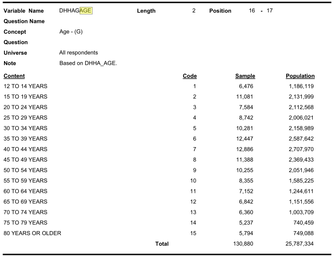
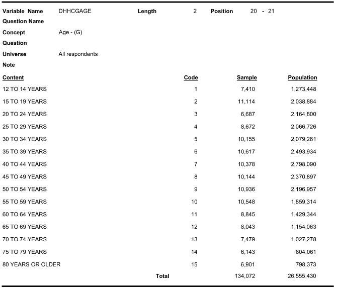
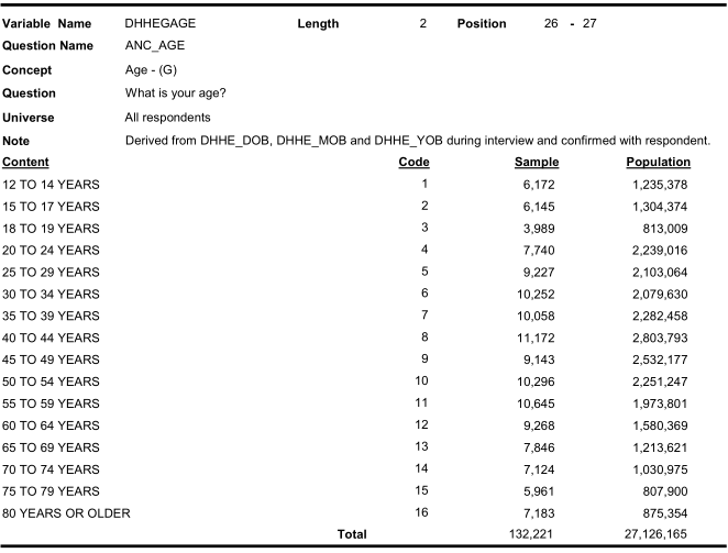
| Age | DHHAGAGE | DHHCGAGE | DHHEGAGE |
| Sex | DHHA_SEX | DHHC_SEX | DHHE_SEX |
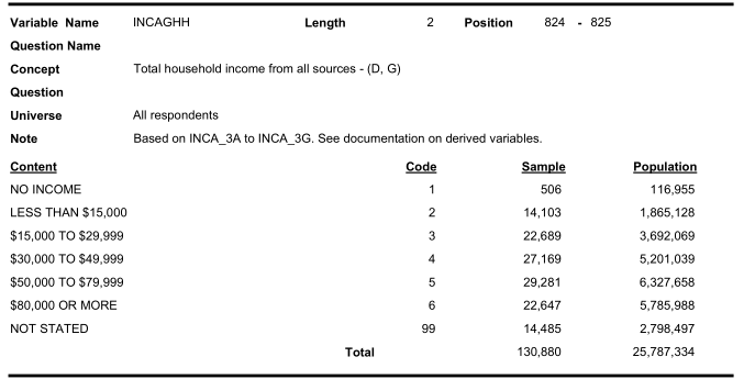
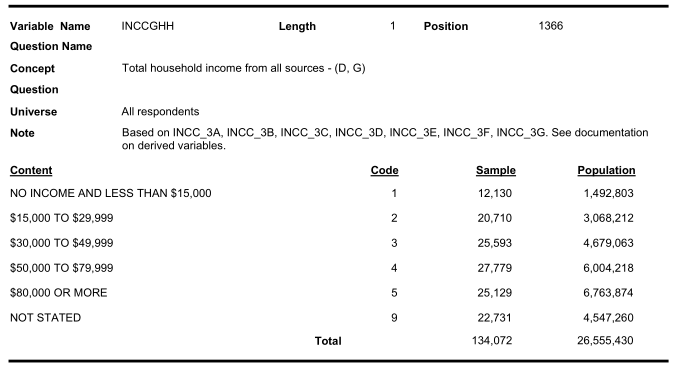
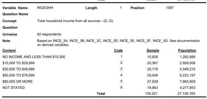
| Household income | INCAGHH | INCCGHH | INCEGHH |
| Cultural/racial origin | SDCAGRAC | SDCCGRAC | SDCEGCGT |
| BMI (Score) | HWTAGBMI | HWTCGBMI | HWTEGBMI |
| BMI (Category) | HWTAGSW | HWTCGISW | HWTEGISW |
| Physical activity | PACADPAI | PACCDPAI | PACEDPAI |
| Smoking status (Type of smoker) | SMKADSTY | SMKCDSTY | SMKEDSTY |
| Fruits/vegetables consumption | FVCADTOT | FVCCDTOT | FVCEDTOT |
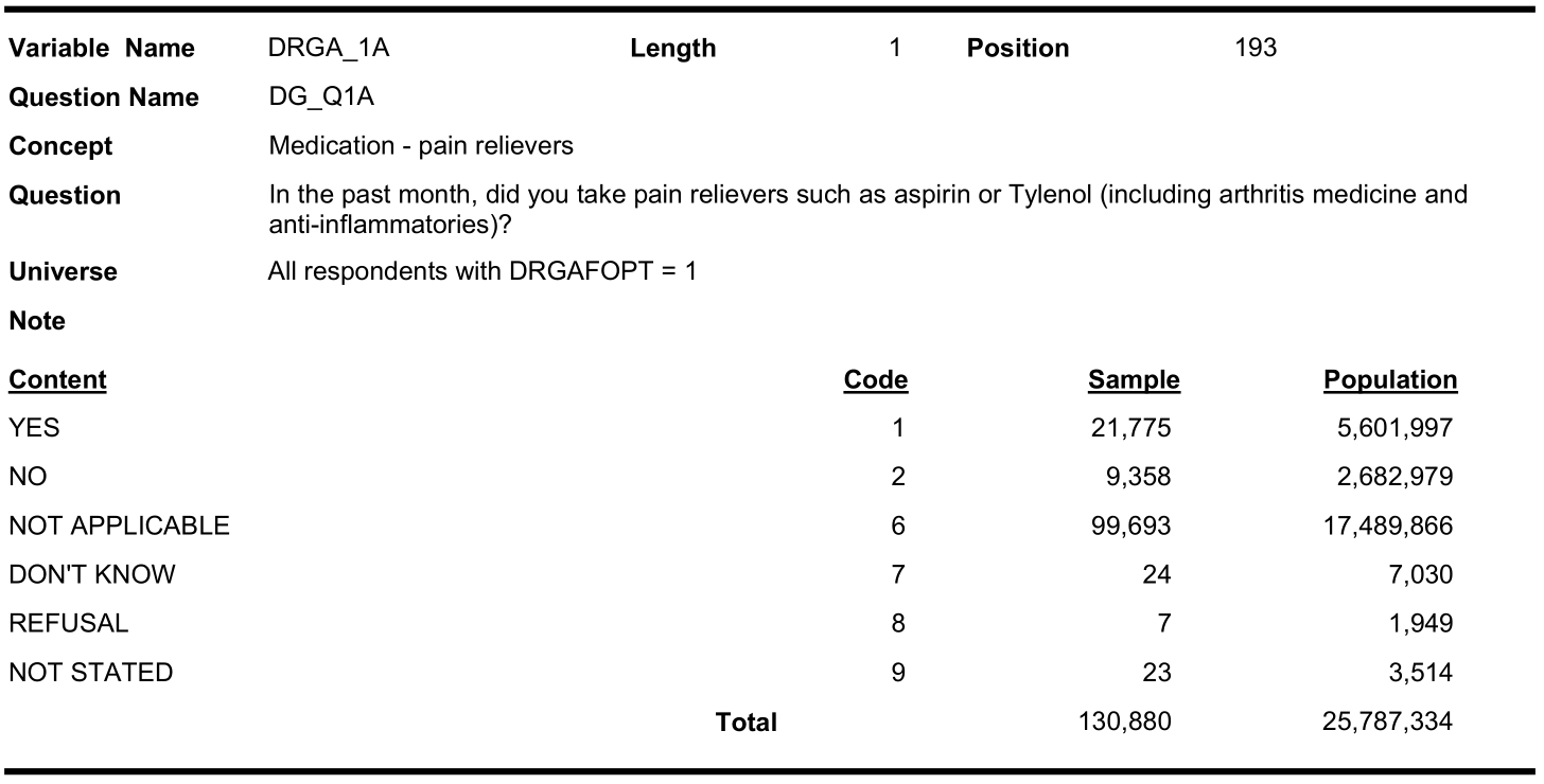
| Pain med use | DRGA_1A | MEDC_1A | MEDE_1A |
| Hypertension | CCCA_071 | CCCC_071 | CCCE_071 |
| Has emphysema or COPD | CCCA_91B | CCCC_91B | CCCE_91F |
| Diabetes | CCCA_101 | CCCC_101 | CCCE_101 |
| Education | EDUADR04 | EDUCDR04 | EDUEDR04 |
| Survey weights | WTSAM | WTSC_M | WTSE_M |
Subset the data
# Restrict the dataset with variables of interest only
var.names1 <- c("CCCA_051", "CCCA_05A", "CCCA_121", "DHHAGAGE",
               "DHHA_SEX", "INCAGHH", "SDCAGRAC", "HWTAGBMI",
               "HWTAGSW", "PACADPAI", "SMKADSTY", "FVCADTOT",
               "DRGA_1A", "CCCA_071", "CCCA_91B", "CCCA_101",
               "EDUADR04", "WTSAM")
cc11 <- c1[var.names1]
dim(cc11)
#> [1] 130880     18
table(cc11$CCCA_051)
#>
#>            YES             NO NOT APPLICABLE     DON'T KNOW        REFUSAL
#>          24511         106231              0            110              3
#>     NOT STATED
#>             25
var.names2 <- c("CCCC_051", "CCCC_05A", "CCCC_121", "DHHCGAGE",
               "DHHC_SEX", "INCCGHH", "SDCCGRAC", "HWTCGBMI",
               "HWTCGISW", "PACCDPAI", "SMKCDSTY", "FVCCDTOT",
               "MEDC_1A", "CCCC_071", "CCCC_91B", "CCCC_101",
               "EDUCDR04", "WTSC_M")
cc21 <- c2[var.names2]
dim(cc21)
#> [1] 134072     18
table(cc21$CCCC_051)
#>
#>            YES             NO NOT APPLICABLE     DON'T KNOW        REFUSAL
#>          29293         104530              0            208             11
#>     NOT STATED
#>             30
var.names3 <- c("CCCE_051", "CCCE_05A", "CCCE_121", "DHHEGAGE",
               "DHHE_SEX", "INCEGHH", "SDCEGCGT", "HWTEGBMI",
               "HWTEGISW", "PACEDPAI", "SMKEDSTY", "FVCEDTOT",
               "MEDE_1A", "CCCE_071", "CCCE_91F", "CCCE_101",
               "EDUEDR04", "WTSE_M")
cc31 <- c3[var.names3]
dim(cc31)
#> [1] 132221     18
table(cc31$CCCE_051)
#>
#>            YES             NO NOT APPLICABLE     DON'T KNOW        REFUSAL
#>          28221         103781              0            191              4
#>     NOT STATED
#>             24
Combine 3 cycle datasets
We want to combine data from three different cycles in order to get more subjects in our data. For that, we will have to stack/append data from three different cycles. In order to do so, we need to make the names exarctly the same. E.g., for BMI category, we will rename all 3 variables: HWTAGSW (from cycle 1), HWTCGISW (from cycle 2) and HWTEGISW (from cycle 3) to bmicat.
Making variable names the same
new.var.names <- c("arthritis", "arthritis.kind", "CVD", "age",
               "sex", "income", "race", "bmi",
               "bmicat", "phyact", "smoke", "fruit",
               "painmed", "ht", "copd", "diab",
               "edu", "weight")
names(cc11) <- names(cc21) <- names(cc31) <- new.var.names

table(cc11$arthritis)
#>
#>            YES             NO NOT APPLICABLE     DON'T KNOW        REFUSAL
#>          24511         106231              0            110              3
#>     NOT STATED
#>             25
table(cc21$arthritis)
#>
#>            YES             NO NOT APPLICABLE     DON'T KNOW        REFUSAL
#>          29293         104530              0            208             11
#>     NOT STATED
#>             30
table(cc31$arthritis)
#>
#>            YES             NO NOT APPLICABLE     DON'T KNOW        REFUSAL
#>          28221         103781              0            191              4
#>     NOT STATED
#>             24
Notice the difference in categorization
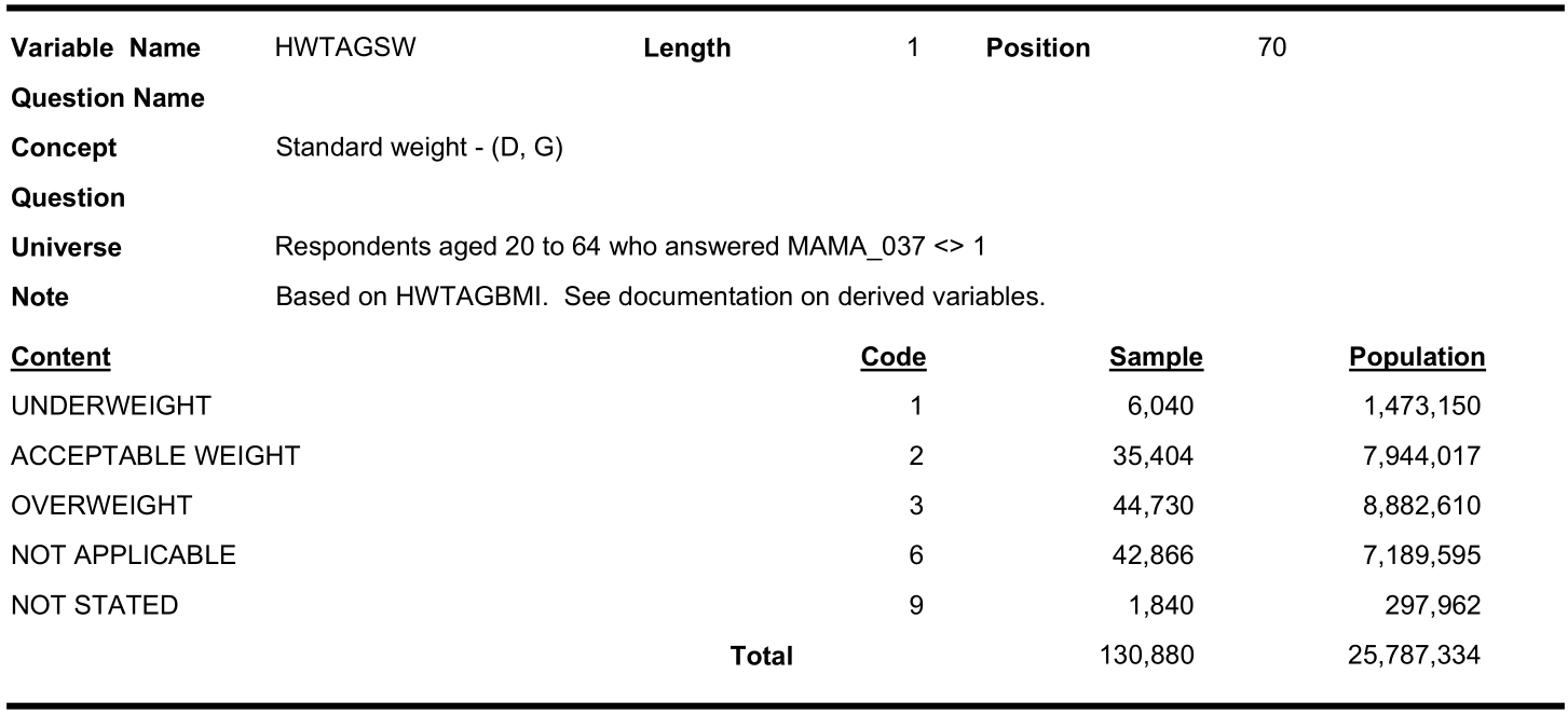
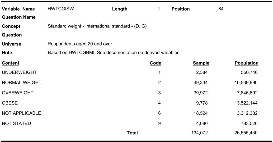
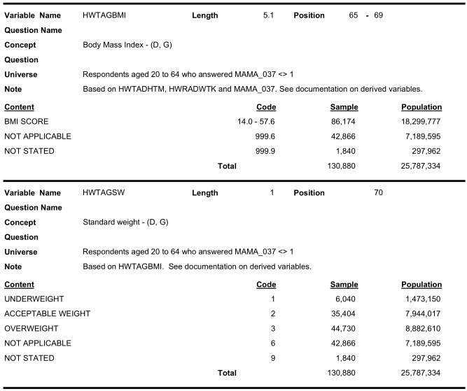
Note that, not only the names of the variables are different, sometimes, the categorization labels are also different. Note the BMI (Category) in the three cycles: HWTAGSW from cycle 1:
HWTCGISW from cycle 2:
HWTEGISW from cycle 3:

table(cc11$bmicat)
#>
#>    UNDERWEIGHT ACCEPT. WEIGHT     OVERWEIGHT NOT APPLICABLE     NOT STATED
#>           6040          35404          44730          42866           1840
table(cc21$bmicat)
#>
#>    UNDERWEIGHT  NORMAL WEIGHT     OVERWEIGHT          OBESE NOT APPLICABLE
#>           2384          49334          39972          19778          18524
#>     DON'T KNOW        REFUSAL     NOT STATED
#>              0              0           4080
table(cc31$bmicat)
#>
#>    UNDERWEIGHT  NORMAL WEIGHT     OVERWEIGHT          OBESE NOT APPLICABLE
#>           2918          51970          40082          20817          12317
#>     DON'T KNOW        REFUSAL     NOT STATED
#>              0              0           4117
In cycle 1.1, the second response (code 2) label was named as “Acceptable weight” where as in cycles 2.1 and 3.1 it was named as “Normal weight”. Also “obese” category was not present in cycle 1.1.
Similarly look for age categories:
Similarly look for income categories:
Therefore, we need to recode the variable value labels carefully.
Appending
Below we append all the three cycles of data:
Subsetting according to eligibility criteria
Criteria 1: control group
Exposure group is people with osteoarthritis. The control group is people who do not have osteoarthritis.
In cycle 1, there were 2 related questions: - Do you have arthritis or rheumatism excluding fibromyalgia? (variable arthritis) - What kind of arthritis do you have? (variable arthritis.kind)
table(cc123a$arthritis)
#>
#>            YES             NO NOT APPLICABLE     DON'T KNOW        REFUSAL
#>          82025         314542              0            509             18
#>     NOT STATED
#>             79
table(cc123a$arthritis.kind)
#>
#> RHEUMATOID ARTH  OSTEOARTHRITIS           OTHER  NOT APPLICABLE      DON'T KNOW
#>           19099           40943            7305          314542           12354
#>         REFUSAL      NOT STATED      RHEUMATISM
#>             215             619            2096
dim(cc123a)
#> [1] 397173     18
In the control group, we do not want to put people with other types of arthritis.
c123sub1 <- subset(cc123a, arthritis.kind == "OSTEOARTHRITIS" |
                    arthritis.kind == "NOT APPLICABLE" )
dim(c123sub1)
#> [1] 355485     18
table(c123sub1$arthritis.kind)
#>
#> RHEUMATOID ARTH  OSTEOARTHRITIS           OTHER  NOT APPLICABLE      DON'T KNOW
#>               0           40943               0          314542               0
#>         REFUSAL      NOT STATED      RHEUMATISM
#>               0               0               0
table(c123sub1$arthritis)
#>
#>            YES             NO NOT APPLICABLE     DON'T KNOW        REFUSAL
#>          40943         314542              0              0              0
#>     NOT STATED
#>              0
require(car)
#> Loading required package: car
#> Loading required package: carData
c123sub1$arthritis.kind <- recode(c123sub1$arthritis.kind,
                        "'OSTEOARTHRITIS'='OA';
                         'NOT APPLICABLE'='Control';
                         else=NA",
                         as.factor = FALSE)
table(c123sub1$arthritis.kind, useNA = "always")
#>
#> Control      OA    <NA>
#>  314542   40943       0
c123sub1$OA <- c123sub1$arthritis.kind
c123sub1$arthritis.kind <- NULL
c123sub1$arthritis <- NULL
Criteria 2: retain valid responses for outcome
table(c123sub1$CVD)
#>
#>            YES             NO NOT APPLICABLE     DON'T KNOW        REFUSAL
#>          19177         336021              0            252             35
#>     NOT STATED
#>              0
c123sub2 <- subset(c123sub1, CVD == "YES" | CVD == "NO")
table(c123sub2$CVD)
#>
#>            YES             NO NOT APPLICABLE     DON'T KNOW        REFUSAL
#>          19177         336021              0              0              0
#>     NOT STATED
#>              0
dim(c123sub2)
#> [1] 355198     17
c123sub2$CVD <- recode(c123sub2$CVD,
                        "'YES'='event';
                         'NO'='0 event';
                         else=NA",
                         as.factor = FALSE)
table(c123sub2$CVD, useNA = "always")
#>
#> 0 event   event    <NA>
#>  336021   19177       0
Criteria 3: Is there a zero cell?
Check out ‘Universe’ for all the variables under consideration. Is there a possibility that cross-tabulation of some of the categories will produce zero?
For example, the ‘Universe’ for BMI or BMI category includes ‘Respondents aged 20 to 64’.
Therefore, we will not have BMI from anyone aged less than 20 or over 64.
table(c123sub2$bmicat, c123sub2$age)[,1:2]
#>
#>                  12 TO 14 YEARS 15 TO 19 YEARS
#>   UNDERWEIGHT                 0              0
#>   ACCEPT. WEIGHT              0              0
#>   OVERWEIGHT                  0              0
#>   NOT APPLICABLE          19934          21891
#>   NOT STATED                  0              0
#>   NORMAL WEIGHT               0              0
#>   OBESE                       0              0
#>   DON'T KNOW                  0              0
#>   REFUSAL                     0              0
# Note the categories of bmicat (duplicate categories)
Also, we check the prevalence of OA and CVD for subjects less than 20 years of age: not a lot of people (still potential for a sensitivity analysis).
table(c123sub2$OA, c123sub2$age)
#>
#>           12 TO 14 YEARS 15 TO 19 YEARS 20 TO 24 YEARS 25 TO 29 YEARS
#>   Control          19927          21795          21303          25490
#>   OA                   7             96            191            345
#>
#>           30 TO 34 YEARS 35 TO 39 YEARS 40 TO 44 YEARS 45 TO 49 YEARS
#>   Control          28851          30359          30267          25302
#>   OA                 595           1027           1639           2482
#>
#>           50 TO 54 YEARS 55 TO 59 YEARS 60 TO 64 YEARS 65 TO 69 YEARS
#>   Control          23670          20036          15751          13024
#>   OA                3988           4991           5093           5257
#>
#>           70 TO 74 YEARS 75 TO 79 YEARS 80 YEARS OR MORE NOT APPLICABLE
#>   Control          11011           8426             9127              0
#>   OA                5236           4671             5227              0
#>
#>           DON'T KNOW REFUSAL NOT STATED 15 TO 17 YEARS 18 TO 19 YEARS
#>   Control          0       0          0           6084           3907
#>   OA               0       0          0              8             15
table(c123sub2$CVD, c123sub2$age)
#>
#>           12 TO 14 YEARS 15 TO 19 YEARS 20 TO 24 YEARS 25 TO 29 YEARS
#>   0 event          19853          21776          21354          25670
#>   event               81            115            140            165
#>
#>           30 TO 34 YEARS 35 TO 39 YEARS 40 TO 44 YEARS 45 TO 49 YEARS
#>   0 event          29237          31090          31378          27049
#>   event              209            296            528            735
#>
#>           50 TO 54 YEARS 55 TO 59 YEARS 60 TO 64 YEARS 65 TO 69 YEARS
#>   0 event          26506          23290          18762          15789
#>   event             1152           1737           2082           2492
#>
#>           70 TO 74 YEARS 75 TO 79 YEARS 80 YEARS OR MORE NOT APPLICABLE
#>   0 event          13375          10229            10703              0
#>   event             2872           2868             3651              0
#>
#>           DON'T KNOW REFUSAL NOT STATED 15 TO 17 YEARS 18 TO 19 YEARS
#>   0 event          0       0          0           6066           3894
#>   event            0       0          0             26             28
Accordingly, we will restrict our analysis (and aim) to adult target population only (age 20 and +). For that, first, recode the age variable, and then exclude the teen category.
# CCHS cycle 1.1 has: '15 TO 19 YEARS'
# Other cycles have: '15 TO 17 YEARS', '18 TO 19 YEARS'
c123sub2$age <- recode(c123sub2$age,
                        "c('12 TO 14 YEARS','15 TO 19 YEARS',
                         '15 TO 17 YEARS', '18 TO 19 YEARS')='teen';
                         c('20 TO 24 YEARS','25 TO 29 YEARS',
                           '30 TO 34 YEARS','35 TO 39 YEARS')='20-39 years';
                         c('40 TO 44 YEARS','45 TO 49 YEARS')='40-49 years';
                         c('50 TO 54 YEARS','55 TO 59 YEARS')='50-59 years';
                         c('60 TO 64 YEARS')='60-64 years';
                         else='65 years and over'",
                         as.factor = FALSE)
table(c123sub2$age)
#>
#>       20-39 years       40-49 years       50-59 years       60-64 years
#>            108161             59690             52685             20844
#> 65 years and over              teen
#>             61979             51839
dim(c123sub2)
#> [1] 355198     17
c123sub3 <- subset(c123sub2, age != 'teen' &
                     age != '65 years and over')
table(c123sub3$age, useNA = "always")
#>
#> 20-39 years 40-49 years 50-59 years 60-64 years        <NA>
#>      108161       59690       52685       20844           0
dim(c123sub3)
#> [1] 241380     17
Criteria 4: Assign missing to the invalid covariate responses
We have invalid covariate responses, such as refused, not ascertained, and don’t know responses. Let’s assign missing values for these invalid responses.
# sex
table(c123sub3$sex)
#>
#>           MALE         FEMALE NOT APPLICABLE     NOT STATED     DON'T KNOW
#>         114104         127276              0              0              0
#>        REFUSAL
#>              0
c123sub3$sex <- car::recode(c123sub3$sex,
                        "'MALE'='Male';
                         'FEMALE' = 'Female';
                         else = NA",
                         as.factor = FALSE)
table(c123sub3$sex, useNA = "always")
#>
#> Female   Male   <NA>
#> 127276 114104      0
# Race
table(c123sub3$race)
#>
#>            WHITE VISIBLE MINORITY   NOT APPLICABLE       NOT STATED
#>           210307            25840                0             5233
#>       DON'T KNOW          REFUSAL
#>                0                0
c123sub3$race <- car::recode(c123sub3$race,
                        "'WHITE'='White';
                         'VISIBLE MINORITY' = 'Non-white';
                         else = NA",
                         as.factor = FALSE)
table(c123sub3$race, useNA = "always")
#>
#> Non-white     White      <NA>
#>     25840    210307      5233

# income
table(c123sub3$income)
#>
#>        NO INCOME LESS THAN 15,000  $15,000-$29,999  $30,000-$49,999
#>             5953             6985            29888            49496
#>  $50,000-$79,999  $80,000 OR MORE   NOT APPLICABLE       NOT STATED
#>            61093            57056                0            25730
#>       DON'T KNOW          REFUSAL   NO OR <$15,000
#>                0                0             5179
# cycle 1.1 has: 'NO INCOME','LESS THAN 15,000'
# Other cycles have: 'NO OR <$15,000'
c123sub3$income <- car::recode(c123sub3$income,
                        "c('NO OR <$15,000', 'NO INCOME',
                        'LESS THAN 15,000',
                        '$15,000-$29,999')='$29,999 or less';
                        '$30,000-$49,999' = '$30,000-$49,999';
                        '$50,000-$79,999' = '$50,000-$79,999';
                        '$80,000 OR MORE' = '$80,000 or more';
                        else = NA",
                          as.factor = FALSE)
table(c123sub3$income, useNA = "always")
#>
#> $29,999 or less $30,000-$49,999 $50,000-$79,999 $80,000 or more            <NA>
#>           48005           49496           61093           57056           25730
# BMI
table(c123sub3$bmicat)
#>
#>    UNDERWEIGHT ACCEPT. WEIGHT     OVERWEIGHT NOT APPLICABLE     NOT STATED
#>           8964          33100          93107           1038           7577
#>  NORMAL WEIGHT          OBESE     DON'T KNOW        REFUSAL
#>          70278          27316              0              0
c123sub3$bmicat <- car::recode(c123sub3$bmicat,
                        "'UNDERWEIGHT'='Underweight';
                         c('ACCEPT. WEIGHT','NORMAL WEIGHT')='Normal';
                         c('OVERWEIGHT','OBESE') = 'Overweight';
                         else = NA",
                         as.factor = FALSE)
table(c123sub3$bmicat, useNA = "always")
#>
#>      Normal  Overweight Underweight        <NA>
#>      103378      120423        8964        8615
c123sub3$bmi <- NULL # no need of the original BMI values
# physical activity
table(c123sub3$phyact)
#>
#>         ACTIVE       MODERATE       INACTIVE NOT APPLICABLE     NOT STATED
#>          57033          60164         117516              0           6667
#>     DON'T KNOW        REFUSAL
#>              0              0
c123sub3$phyact <- car::recode(c123sub3$phyact,
                        "'ACTIVE'='Active';
                         'MODERATE' = 'Moderate';
                         'INACTIVE' = 'Inactive';
                         else = NA",
                         as.factor = FALSE)
table(c123sub3$phyact, useNA = "always")
#>
#>   Active Inactive Moderate     <NA>
#>    57033   117516    60164     6667
# smoking
table(c123sub3$smoke)
#>
#>            DAILY       OCCASIONAL ALWAYS OCCASION.     FORMER DAILY
#>            58747             8175             4399            59722
#> FORMER OCCASION.     NEVER SMOKED   NOT APPLICABLE       NOT STATED
#>            38123            71397                0              817
#>       DON'T KNOW          REFUSAL
#>                0                0
c123sub3$smoke <- car::recode(c123sub3$smoke,
                        "c('DAILY','OCCASIONAL',
                           'ALWAYS OCCASION.')='Current smoker';
                         c('FORMER DAILY','FORMER OCCASION.') = 'Former smoker';
                         'NEVER SMOKED' = 'Never smoker';
                         else = NA",
                         as.factor = FALSE)
table(c123sub3$smoke, useNA = "always")
#>
#> Current smoker  Former smoker   Never smoker           <NA>
#>          71321          97845          71397            817
# fruit and vegetable consumption
str(c123sub3$fruit)
#>  Factor w/ 303 levels "0","0.1","0.2",..: 42 67 39 61 51 51 48 41 17 27 ...
c123sub3$fruit.cont <- c123sub3$fruit
c123sub3$fruit2 <- as.numeric(as.character(c123sub3$fruit))
#> Warning: NAs introduced by coercion
# Note: do not use as.numeric(c123sub3$fruit)
summary(c123sub3$fruit2)
#>    Min. 1st Qu.  Median    Mean 3rd Qu.    Max.    NA's
#>   0.000   2.900   4.100   4.627   5.900  64.300   42987
c123sub3$fruit2 <- cut(c123sub3$fruit2,
                      breaks = c(0,3,6,Inf),
                      right = TRUE,
                      include.lowest = TRUE,
                      labels = c("0-3 daily serving",
                                 "4-6 daily serving",
                                 ">6 daily serving"))
table(c123sub3$fruit2, useNA = "always")
#>
#> 0-3 daily serving 4-6 daily serving  >6 daily serving              <NA>
#>             56355             96177             45861             42987
# Sanity check: true zeros must not be dropped to NA by the cut()
fruit.num <- as.numeric(as.character(c123sub3$fruit.cont))
#> Warning: NAs introduced by coercion
stopifnot(all(!is.na(c123sub3$fruit2[!is.na(fruit.num) & fruit.num == 0])))
c123sub3$fruit <- c123sub3$fruit2
c123sub3$fruit2 <- NULL
# pain medication
table(c123sub3$painmed)
#>
#>            YES             NO NOT APPLICABLE     DON'T KNOW        REFUSAL
#>          25743          11141         204323             32             13
#>     NOT STATED
#>            128
c123sub3$painmed <- car::recode(c123sub3$painmed,
                        "'YES'='Yes';
                         'NO' = 'No';
                         else = NA",
                         as.factor = FALSE)
table(c123sub3$painmed, useNA = "always")
#>
#>     No    Yes   <NA>
#>  11141  25743 204496
# hypertension
table(c123sub3$ht)
#>
#>            YES             NO NOT APPLICABLE     DON'T KNOW        REFUSAL
#>          27592         213432              0            331             25
#>     NOT STATED
#>              0
c123sub3$ht <- car::recode(c123sub3$ht,
                        "'YES'='Yes';
                         'NO' = 'No';
                         else = NA",
                         as.factor = FALSE)
table(c123sub3$ht, useNA = "always")
#>
#>     No    Yes   <NA>
#> 213432  27592    356
# COPD
table(c123sub3$copd)
#>
#>            YES             NO NOT APPLICABLE     DON'T KNOW        REFUSAL
#>           1353         192608          47329             70              0
#>     NOT STATED
#>             20
c123sub3$copd <- car::recode(c123sub3$copd,
                        "'YES'='Yes';
                         'NO' = 'No';
                         else = NA",
                         as.factor = FALSE)
table(c123sub3$copd, useNA = "always")
#>
#>     No    Yes   <NA>
#> 192608   1353  47419
# Diabetes
table(c123sub3$diab)
#>
#>            YES             NO NOT APPLICABLE     DON'T KNOW        REFUSAL
#>           8811         232486              0             81              2
#>     NOT STATED
#>              0
c123sub3$diab <- car::recode(c123sub3$diab,
                        "'YES'='Yes';
                         'NO' = 'No';
                         else = NA",
                         as.factor = FALSE)
table(c123sub3$diab, useNA = "always")
#>
#>     No    Yes   <NA>
#> 232486   8811     83
# Education
table(c123sub3$edu)
#>
#> < THAN SECONDARY  SECONDARY GRAD.  OTHER POST-SEC.  POST-SEC. GRAD.
#>            37775            44376            19273           136031
#>   NOT APPLICABLE       NOT STATED       DON'T KNOW          REFUSAL
#>                0             3925                0                0
c123sub3$edu <- car::recode(c123sub3$edu,
                        "'< THAN SECONDARY'='< 2ndary';
                         'SECONDARY GRAD.' = '2nd grad.';
                         'POST-SEC. GRAD.' = 'Post-2nd grad.';
                         'OTHER POST-SEC.' = 'Other 2nd grad.';
                         else = NA",
                         as.factor = FALSE)
table(c123sub3$edu, useNA = "always")
#>
#>        < 2ndary       2nd grad. Other 2nd grad.  Post-2nd grad.            <NA>
#>           37775           44376           19273          136031            3925
Naive Analysis of combined 3 cycles
In the current analysis, we will simply consider all of the variables under consideration as ‘confounders’, and include in our analysis. Later we will perform a refined analysis.
Summary of the analytic data
Including missing values
dim(c123sub3)
#> [1] 241380     17
analytic <- c123sub3
dim(analytic)
#> [1] 241380     17

require("tableone")
#> Loading required package: tableone
CreateTableOne(vars = c("CVD", "age",
               "sex", "income", "race",
               "bmicat", "phyact", "smoke", "fruit",
               "painmed", "ht", "copd", "diab", "edu"),
               data = analytic, includeNA = TRUE)
#>
#>                        Overall
#>   n                    241380
#>   CVD = event (%)        7044 ( 2.9)
#>   age (%)
#>      20-39 years       108161 (44.8)
#>      40-49 years        59690 (24.7)
#>      50-59 years        52685 (21.8)
#>      60-64 years        20844 ( 8.6)
#>   sex = Male (%)       114104 (47.3)
#>   income (%)
#>      $29,999 or less    48005 (19.9)
#>      $30,000-$49,999    49496 (20.5)
#>      $50,000-$79,999    61093 (25.3)
#>      $80,000 or more    57056 (23.6)
#>      NA                 25730 (10.7)
#>   race (%)
#>      Non-white          25840 (10.7)
#>      White             210307 (87.1)
#>      NA                  5233 ( 2.2)
#>   bmicat (%)
#>      Normal            103378 (42.8)
#>      Overweight        120423 (49.9)
#>      Underweight         8964 ( 3.7)
#>      NA                  8615 ( 3.6)
#>   phyact (%)
#>      Active             57033 (23.6)
#>      Inactive          117516 (48.7)
#>      Moderate           60164 (24.9)
#>      NA                  6667 ( 2.8)
#>   smoke (%)
#>      Current smoker     71321 (29.5)
#>      Former smoker      97845 (40.5)
#>      Never smoker       71397 (29.6)
#>      NA                   817 ( 0.3)
#>   fruit (%)
#>      0-3 daily serving  56256 (23.3)
#>      4-6 daily serving  96177 (39.8)
#>      6+ daily serving   45861 (19.0)
#>      NA                 43086 (17.8)
#>   painmed (%)
#>      No                 11141 ( 4.6)
#>      Yes                25743 (10.7)
#>      NA                204496 (84.7)
#>   ht (%)
#>      No                213432 (88.4)
#>      Yes                27592 (11.4)
#>      NA                   356 ( 0.1)
#>   copd (%)
#>      No                192608 (79.8)
#>      Yes                 1353 ( 0.6)
#>      NA                 47419 (19.6)
#>   diab (%)
#>      No                232486 (96.3)
#>      Yes                 8811 ( 3.7)
#>      NA                    83 ( 0.0)
#>   edu (%)
#>      < 2ndary           37775 (15.6)
#>      2nd grad.          44376 (18.4)
#>      Other 2nd grad.    19273 ( 8.0)
#>      Post-2nd grad.    136031 (56.4)
#>      NA                  3925 ( 1.6)
CreateTableOne(vars = c("CVD", "age",
               "sex", "income", "race",
               "bmicat", "phyact", "smoke", "fruit",
               "painmed", "ht", "copd", "diab", "edu"),
               data = analytic, strata = "OA", includeNA = TRUE)
#>                       Stratified by OA
#>                        Control        OA            p      test
#>   n                    221029         20351
#>   CVD = event (%)        5429 ( 2.5)   1615 ( 7.9)  <0.001
#>   age (%)                                           <0.001
#>      20-39 years       106003 (48.0)   2158 (10.6)
#>      40-49 years        55569 (25.1)   4121 (20.2)
#>      50-59 years        43706 (19.8)   8979 (44.1)
#>      60-64 years        15751 ( 7.1)   5093 (25.0)
#>   sex = Male (%)       107729 (48.7)   6375 (31.3)  <0.001
#>   income (%)                                        <0.001
#>      $29,999 or less    42019 (19.0)   5986 (29.4)
#>      $30,000-$49,999    45090 (20.4)   4406 (21.7)
#>      $50,000-$79,999    56754 (25.7)   4339 (21.3)
#>      $80,000 or more    53637 (24.3)   3419 (16.8)
#>      NA                 23529 (10.6)   2201 (10.8)
#>   race (%)                                          <0.001
#>      Non-white          24681 (11.2)   1159 ( 5.7)
#>      White             191513 (86.6)  18794 (92.3)
#>      NA                  4835 ( 2.2)    398 ( 2.0)
#>   bmicat (%)                                        <0.001
#>      Normal             96697 (43.7)   6681 (32.8)
#>      Overweight        107871 (48.8)  12552 (61.7)
#>      Underweight         8490 ( 3.8)    474 ( 2.3)
#>      NA                  7971 ( 3.6)    644 ( 3.2)
#>   phyact (%)                                        <0.001
#>      Active             52942 (24.0)   4091 (20.1)
#>      Inactive          106580 (48.2)  10936 (53.7)
#>      Moderate           55222 (25.0)   4942 (24.3)
#>      NA                  6285 ( 2.8)    382 ( 1.9)
#>   smoke (%)                                         <0.001
#>      Current smoker     65398 (29.6)   5923 (29.1)
#>      Former smoker      88210 (39.9)   9635 (47.3)
#>      Never smoker       66663 (30.2)   4734 (23.3)
#>      NA                   758 ( 0.3)     59 ( 0.3)
#>   fruit (%)                                         <0.001
#>      0-3 daily serving  52140 (23.6)   4116 (20.2)
#>      4-6 daily serving  87951 (39.8)   8226 (40.4)
#>      6+ daily serving   41606 (18.8)   4255 (20.9)
#>      NA                 39332 (17.8)   3754 (18.4)
#>   painmed (%)                                       <0.001
#>      No                 10624 ( 4.8)    517 ( 2.5)
#>      Yes                23084 (10.4)   2659 (13.1)
#>      NA                187321 (84.7)  17175 (84.4)
#>   ht (%)                                            <0.001
#>      No                198550 (89.8)  14882 (73.1)
#>      Yes                22142 (10.0)   5450 (26.8)
#>      NA                   337 ( 0.2)     19 ( 0.1)
#>   copd (%)                                          <0.001
#>      No                173224 (78.4)  19384 (95.2)
#>      Yes                  938 ( 0.4)    415 ( 2.0)
#>      NA                 46867 (21.2)    552 ( 2.7)
#>   diab (%)                                          <0.001
#>      No                213910 (96.8)  18576 (91.3)
#>      Yes                 7046 ( 3.2)   1765 ( 8.7)
#>      NA                    73 ( 0.0)     10 ( 0.0)
#>   edu (%)                                           <0.001
#>      < 2ndary           32884 (14.9)   4891 (24.0)
#>      2nd grad.          40950 (18.5)   3426 (16.8)
#>      Other 2nd grad.    17808 ( 8.1)   1465 ( 7.2)
#>      Post-2nd grad.    125772 (56.9)  10259 (50.4)
#>      NA                  3615 ( 1.6)    310 ( 1.5)
require(DataExplorer)
#> Loading required package: DataExplorer
plot_missing(analytic)
#> Warning: `aes_string()` was deprecated in ggplot2 3.0.0.
#> ℹ Please use tidy evaluation idioms with `aes()`.
#> ℹ See also `vignette("ggplot2-in-packages")` for more information.
#> ℹ The deprecated feature was likely used in the DataExplorer package.
#>   Please report the issue at
#>   <https://github.com/boxuancui/DataExplorer/issues>.
Let us investigate why pain medication has so much missing
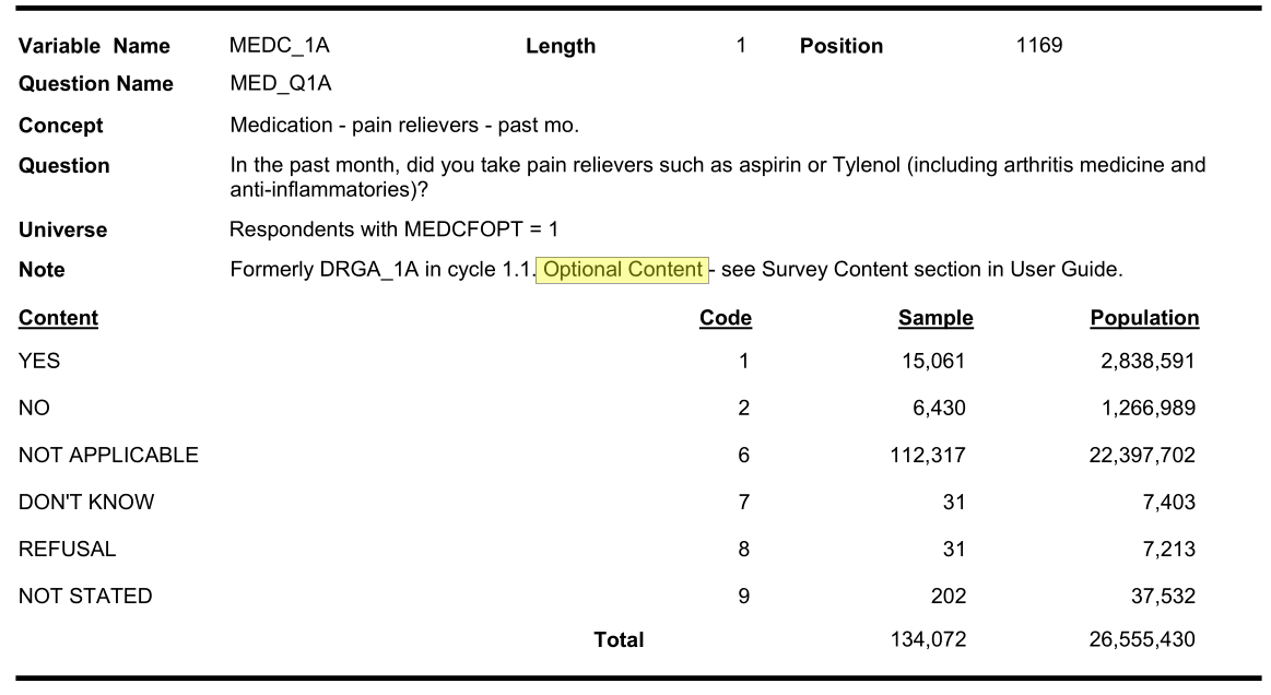
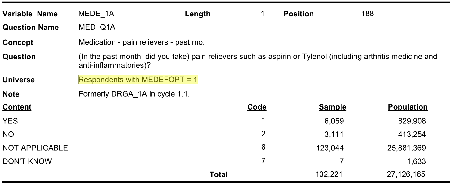
Optional content respondent (cycle 3.1):
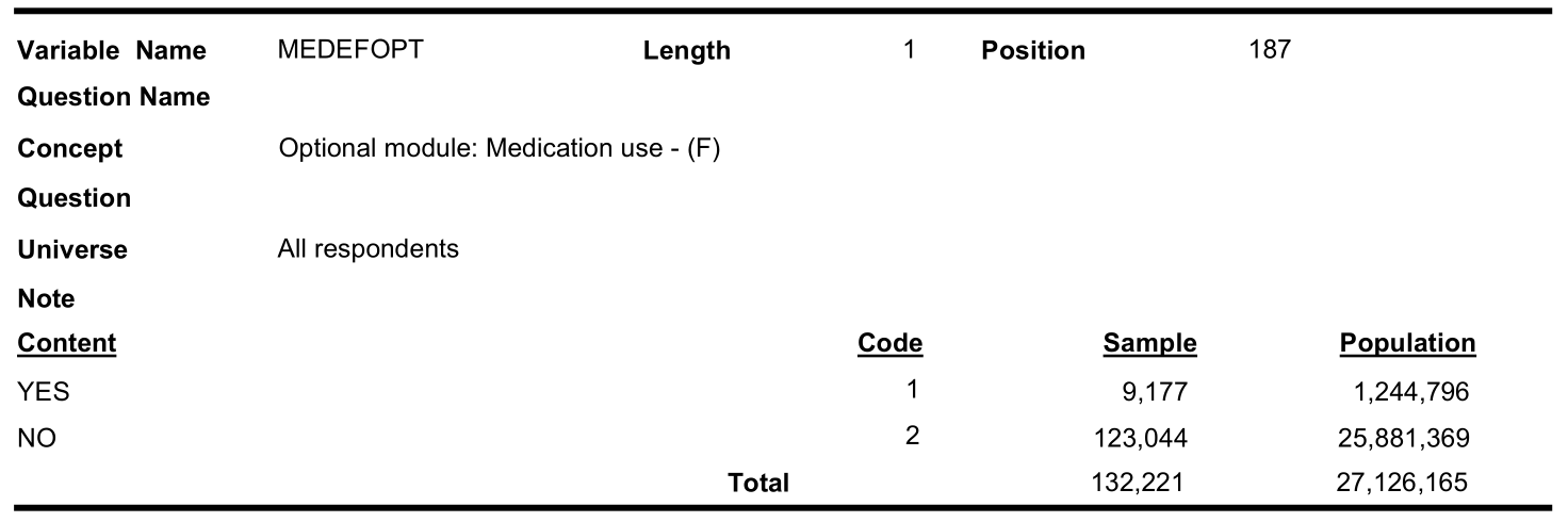
In cycle 2.1, only 21,755 out of 134,072 responded to optional medication component.
Complete case analysis
dim(c123sub3)
#> [1] 241380     17
analytic2 <- as.data.frame(na.omit(c123sub3))
dim(analytic2)
#> [1] 21623    17


tab1 <- CreateTableOne(vars = c("CVD", "age",
               "sex", "income", "race",
               "bmicat", "phyact", "smoke", "fruit",
               "painmed", "ht", "copd", "diab", "edu"),
               data = analytic2, includeNA = TRUE)
print(tab1, showAllLevels = TRUE)
#>
#>               level             Overall
#>   n                             21623
#>   CVD (%)     0 event           20917 (96.7)
#>               event               706 ( 3.3)
#>   age (%)     20-39 years        7119 (32.9)
#>               40-49 years        7024 (32.5)
#>               50-59 years        5457 (25.2)
#>               60-64 years        2023 ( 9.4)
#>   sex (%)     Female            10982 (50.8)
#>               Male              10641 (49.2)
#>   income (%)  $29,999 or less    4054 (18.7)
#>               $30,000-$49,999    4461 (20.6)
#>               $50,000-$79,999    6600 (30.5)
#>               $80,000 or more    6508 (30.1)
#>   race (%)    Non-white          2488 (11.5)
#>               White             19135 (88.5)
#>   bmicat (%)  Normal             8993 (41.6)
#>               Overweight        11739 (54.3)
#>               Underweight         891 ( 4.1)
#>   phyact (%)  Active             5502 (25.4)
#>               Inactive          10495 (48.5)
#>               Moderate           5626 (26.0)
#>   smoke (%)   Current smoker     5887 (27.2)
#>               Former smoker      9368 (43.3)
#>               Never smoker       6368 (29.5)
#>   fruit (%)   0-3 daily serving  5806 (26.9)
#>               4-6 daily serving 10730 (49.6)
#>               6+ daily serving   5087 (23.5)
#>   painmed (%) No                 6197 (28.7)
#>               Yes               15426 (71.3)
#>   ht (%)      No                19014 (87.9)
#>               Yes                2609 (12.1)
#>   copd (%)    No                21475 (99.3)
#>               Yes                 148 ( 0.7)
#>   diab (%)    No                20760 (96.0)
#>               Yes                 863 ( 4.0)
#>   edu (%)     < 2ndary           2998 (13.9)
#>               2nd grad.          4605 (21.3)
#>               Other 2nd grad.    1509 ( 7.0)
#>               Post-2nd grad.    12511 (57.9)
tab1b <- CreateTableOne(vars = c("CVD", "age",
               "sex", "income", "race",
               "bmicat", "phyact", "smoke", "fruit",
               "painmed", "ht", "copd", "diab", "edu"),
               data = analytic2, strata = "OA", includeNA = TRUE)
print(tab1b, showAllLevels = TRUE)
#>              Stratified by OA
#>               level             Control       OA           p      test
#>   n                             19459         2164
#>   CVD (%)     0 event           18917 (97.2)  2000 (92.4)  <0.001
#>               event               542 ( 2.8)   164 ( 7.6)
#>   age (%)     20-39 years        6915 (35.5)   204 ( 9.4)  <0.001
#>               40-49 years        6515 (33.5)   509 (23.5)
#>               50-59 years        4504 (23.1)   953 (44.0)
#>               60-64 years        1525 ( 7.8)   498 (23.0)
#>   sex (%)     Female             9521 (48.9)  1461 (67.5)  <0.001
#>               Male               9938 (51.1)   703 (32.5)
#>   income (%)  $29,999 or less    3413 (17.5)   641 (29.6)  <0.001
#>               $30,000-$49,999    3968 (20.4)   493 (22.8)
#>               $50,000-$79,999    6023 (31.0)   577 (26.7)
#>               $80,000 or more    6055 (31.1)   453 (20.9)
#>   race (%)    Non-white          2370 (12.2)   118 ( 5.5)  <0.001
#>               White             17089 (87.8)  2046 (94.5)
#>   bmicat (%)  Normal             8277 (42.5)   716 (33.1)  <0.001
#>               Overweight        10356 (53.2)  1383 (63.9)
#>               Underweight         826 ( 4.2)    65 ( 3.0)
#>   phyact (%)  Active             4986 (25.6)   516 (23.8)   0.190
#>               Inactive           9417 (48.4)  1078 (49.8)
#>               Moderate           5056 (26.0)   570 (26.3)
#>   smoke (%)   Current smoker     5247 (27.0)   640 (29.6)  <0.001
#>               Former smoker      8363 (43.0)  1005 (46.4)
#>               Never smoker       5849 (30.1)   519 (24.0)
#>   fruit (%)   0-3 daily serving  5290 (27.2)   516 (23.8)  <0.001
#>               4-6 daily serving  9686 (49.8)  1044 (48.2)
#>               6+ daily serving   4483 (23.0)   604 (27.9)
#>   painmed (%) No                 5859 (30.1)   338 (15.6)  <0.001
#>               Yes               13600 (69.9)  1826 (84.4)
#>   ht (%)      No                17356 (89.2)  1658 (76.6)  <0.001
#>               Yes                2103 (10.8)   506 (23.4)
#>   copd (%)    No                19359 (99.5)  2116 (97.8)  <0.001
#>               Yes                 100 ( 0.5)    48 ( 2.2)
#>   diab (%)    No                18751 (96.4)  2009 (92.8)  <0.001
#>               Yes                 708 ( 3.6)   155 ( 7.2)
#>   edu (%)     < 2ndary           2527 (13.0)   471 (21.8)  <0.001
#>               2nd grad.          4173 (21.4)   432 (20.0)
#>               Other 2nd grad.    1364 ( 7.0)   145 ( 6.7)
#>               Post-2nd grad.    11395 (58.6)  1116 (51.6)
Save data for later
References
Rahman, M Mushfiqur, Jacek A Kopec, Jolanda Cibere, Charlie H Goldsmith, and Aslam H Anis. 2013. “The Relationship Between Osteoarthritis and Cardiovascular Disease in a Population Health Survey: A Cross-Sectional Study.” BMJ Open 3 (5): e002624.