NHANES: Subsetting

The tutorial demonstrates how to work with subset of complex survey data, specifically focusing on an NHANES example.

The required packages are loaded.

# Load required packages
library(survey)
library(Publish)
library(DataExplorer)

Load data

Survey data is loaded into the R environment.

load("Data/surveydata/NHANES17.RData")
ls()
#> [1] "analytic"           "analytic.with.miss" "has_annotations"

Check missingness

A subset of variables is selected, and the presence of missing data is visualized.

Vars <- c("ID", 
          "weight", 
          "psu", 
          "strata", 
          "gender", 
          "born", 
          "race", 
          "bmi", 
          "cholesterol", 
          "diabetes")
analytic.full.data <- analytic.with.miss[,Vars]

A new variable is also created to categorize cholesterol levels as “healthy” or “unhealthy.”

analytic.full.data$cholesterol.bin <- ifelse(analytic.full.data$cholesterol <200, "healthy", "unhealthy")
analytic.full.data$cholesterol <- NULL

require(DataExplorer)
plot_missing(analytic.full.data)

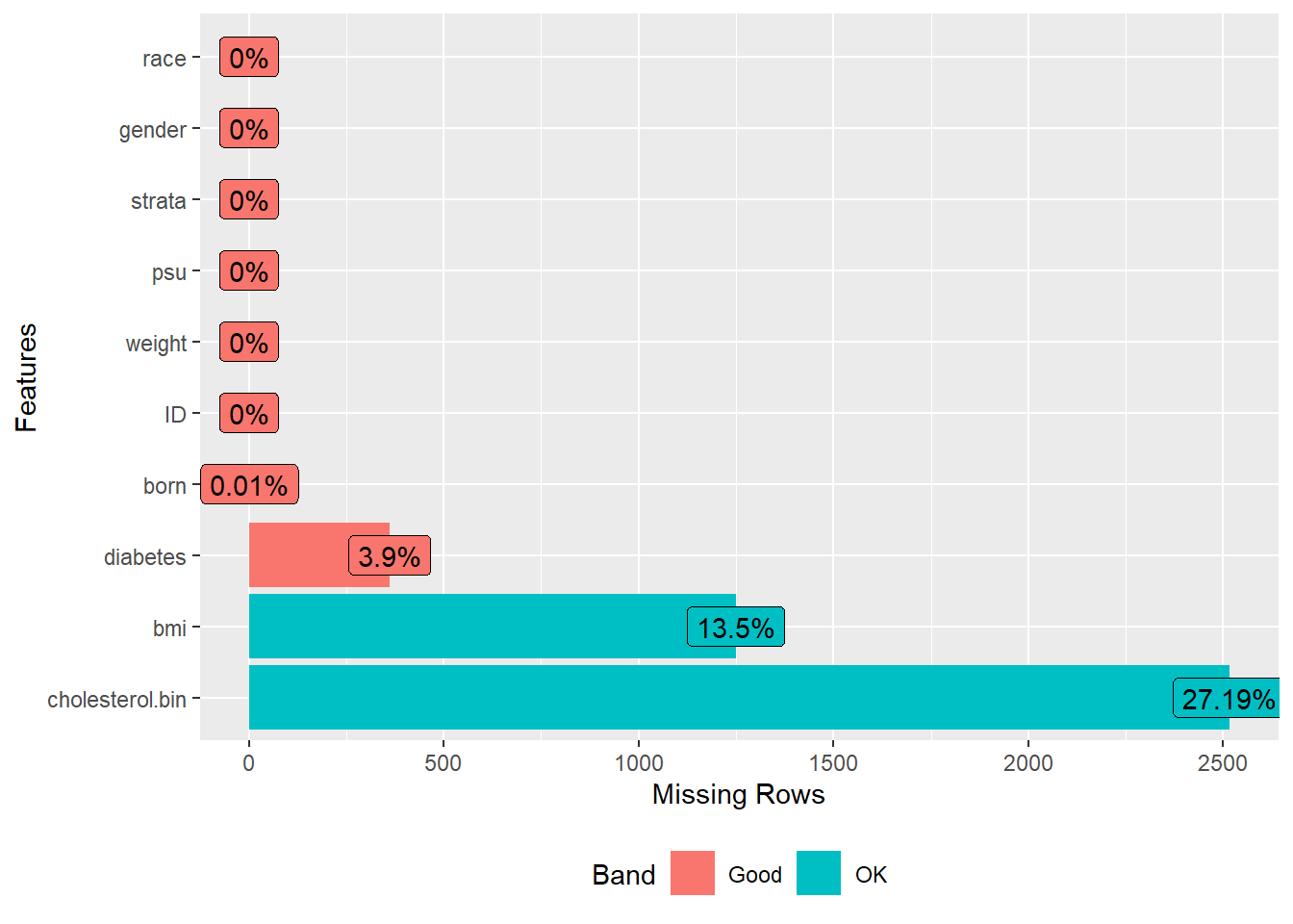
Subsetting Complex Survey data

We are subsetting based on whether the subjects have missing observation (e.g., only retaining those with complete information). This is often an eligibility criteria in studies. In missing data analysis, we will learn more about more appropriate approaches.

dim(analytic.full.data)
#> [1] 9254   10
head(analytic.full.data$ID) # full data
#> [1] 93703 93704 93705 93706 93707 93708
analytic.complete.case.only <- as.data.frame(na.omit(analytic.full.data))
dim(analytic.complete.case.only)
#> [1] 6636   10
head(analytic.complete.case.only$ID) # complete case
#> [1] 93705 93706 93707 93708 93709 93711
head(analytic.full.data$ID[analytic.full.data$ID %in% analytic.complete.case.only$ID])
#> [1] 93705 93706 93707 93708 93709 93711

Below we show how to identify who has missing observations vs not based on full (analytic.full.data) and complete case (analytic.complete.case.only) data. See Heeringa et al (2010) book page 114 (section 4.5.3 “Preparation for Subclass analyses”) and also page 218 (section 7.5.4 “appropriate analysis: incorporating all Sample Design Features”). This is done for 2 reasons:

• full complex survey design structure is taken into account, so that variance estimation is done correctly. If one or more PSU were excluded because none of the complete cases were observed in those PSU, the sub-population (complete cases) will not have complete information of how many PSU were actually present in the original complex design. Then in the population, a reduced number of PSUs would be used to calculate variance (number of SPU is a component of the variance calculation formula, see equation (5.2) in Heeringa et al (2010) textbook. Same is true for strata.), and will result in a wrong/biased variance estimate. Also see West et al. doi: 10.1177/1536867X0800800404
• size of sub-population (here, those with complete cases) is recognized as a random variable; not just a fixed size.

# assign missing indicator
analytic.full.data$miss <- 1 
# assign missing indicator = 0 if the observation is available
analytic.full.data$miss[analytic.full.data$ID %in% analytic.complete.case.only$ID] <- 0

table(analytic.full.data$miss)
#> 
#>    0    1 
#> 6636 2618
# IDs not in complete case data
head(analytic.full.data$ID[analytic.full.data$miss==1])
#> [1] 93703 93704 93710 93720 93724 93725
# IDs in complete case data
head(analytic.full.data$ID[analytic.full.data$miss==0])
#> [1] 93705 93706 93707 93708 93709 93711

Logistic regression on sub-population

A logistic regression model is run on the subset of data that has no missing values. Here, it distinguishes between correct and incorrect approaches to account for the complex survey design.

require(survey)
require(Publish)
model.formula <- as.formula("I(cholesterol.bin=='healthy')~
                            diabetes+gender+born+race+bmi")

Wrong approach

w.design.wrong <- svydesign(ids=~psu, 
                       weights=~weight, 
                       strata=~strata,
                       data = analytic.complete.case.only, #wrong!!
                       nest = TRUE)

Correct approach

w.design0 <- svydesign(ids=~psu, 
                       weights=~weight, 
                       strata=~strata,
                       data = analytic.full.data, 
                       nest = TRUE)

# retain only those that have complete observation / no missing
w.design <- subset(w.design0, miss == 0)# this is the subset design

Full model

fit <- svyglm(model.formula, family = quasibinomial, 
              design = w.design) # subset design
publish(fit)
#>  Variable                            Units Coefficient           CI.95     p-value 
#>  diabetes                               No         Ref                             
#>                                        Yes        0.38     [0.20;0.57]   0.0049202 
#>    gender                           Female         Ref                             
#>                                       Male        0.22     [0.03;0.40]   0.0568343 
#>      born Born in 50 US states or Washingt         Ref                             
#>                                     Others       -0.66   [-0.84;-0.47]   0.0002304 
#>                                    Refused      -12.26 [-13.65;-10.88]     < 1e-04 
#>      race                            Black         Ref                             
#>                                   Hispanic        0.20    [-0.08;0.47]   0.2075536 
#>                                      Other       -0.17    [-0.38;0.03]   0.1439474 
#>                                      White       -0.37   [-0.66;-0.09]   0.0355030 
#>       bmi                                        -0.04   [-0.05;-0.02]   0.0007697

Variable selection

Finally, we discuss variable selection methods. We employ backward elimination to determine which variables are significant predictors while retaining an important variable in the model. If unsure about usefulness of some (gender, born, race, bmi) variables in predicting the outcome, check via backward elimination while keeping important variable (diabetes, say, that has been established in the literature) in the model

model.formula <- as.formula("I(cholesterol.bin=='healthy')~
                            diabetes+gender+born+race+bmi")

scope <- list(upper = ~ diabetes+gender+born+race+bmi, lower = ~ diabetes)

fit <- svyglm(model.formula, design=w.design, # subset design
              family=quasibinomial)

fitstep <- step(fit,  scope = scope, trace = FALSE, direction = "backward")
publish(fitstep) # final model
#>  Variable                            Units Coefficient           CI.95     p-value 
#>  diabetes                               No         Ref                             
#>                                        Yes        0.38     [0.20;0.57]   0.0049202 
#>    gender                           Female         Ref                             
#>                                       Male        0.22     [0.03;0.40]   0.0568343 
#>      born Born in 50 US states or Washingt         Ref                             
#>                                     Others       -0.66   [-0.84;-0.47]   0.0002304 
#>                                    Refused      -12.26 [-13.65;-10.88]     < 1e-04 
#>      race                            Black         Ref                             
#>                                   Hispanic        0.20    [-0.08;0.47]   0.2075536 
#>                                      Other       -0.17    [-0.38;0.03]   0.1439474 
#>                                      White       -0.37   [-0.66;-0.09]   0.0355030 
#>       bmi                                        -0.04   [-0.05;-0.02]   0.0007697

Also see (Stata 2023) for further details.

Video content (optional)

Tip

For those who prefer a video walkthrough, feel free to watch the video below, which offers a description of an earlier version of the above content.

References

Stata. 2023. “How Can i Analyze a Subpopulation of My Survey Data in Stata?” https://stats.oarc.ucla.edu/stata/faq/how-can-i-analyze-a-subpopulation-of-my-survey-data-in-stata/.