PSM in OA-CVD (CCHS)
This tutorial is a comprehensive guide on implementing Propensity Score Matching (PSM) using R, particularly focusing on a OA - CVD health study from the Canadian Community Health Survey (CCHS). This PSM method is used to reduce bias due to confounding variables in observational studies by matching treated and control units with similar propensity scores. The tutorial illustrates that PSM is an iterative process, where researchers may need to refine their matching strategy to achieve satisfactory balance in the matched sample. Different strategies for estimating the treatment effect in the matched sample are explored, each with its own assumptions and implications.
Load packages
At first, various R packages are loaded to utilize their functions for data manipulation, statistical analysis, and visualization.
Load data
The dataset is loaded into the R environment. Variables are renamed to avoid conflicts in subsequent analyses.
Analysis
We are going to apply propensity score analysis (Matching) in our OA - CVD problem from CCHS. For computation considerations, we will only work with cycle 1.1, and the people from Northern provinces in Canada (analytic11n data).
Step 1
Specify PS
A logistic regression model formula is specified to calculate the propensity scores (PS), which is the probability of receiving the treatment given the observed covariates.
ps.formula <- as.formula("OA ~ age + sex + stress + married +
                         income + race + bmi + phyact + smoke +
                        doctor + drink + bp +
                         immigrate + fruit + diab + edu")
var.names <- c("age", "sex", "stress", "married",
               "income", "race", "bmi", "phyact", "smoke",
               "doctor", "drink", "bp",
               "immigrate", "fruit", "diab", "edu")
Fit model
The software fits the PS model using a logistic regression by default. This package actually performs step 1 and 2 with one command matchit.
Look at the documentation for arguments of matchit (RDocumentation 2023) (see also ?matchit). In the current MatchIt (v4.x) API the main signature is:
matchit(formula, data, method = "nearest", distance = "glm",
        link = "logit", distance.options = list(), estimand = "ATT",
        exact = NULL, mahvars = NULL, antiexact = NULL, discard = "none",
        reestimate = FALSE, s.weights = NULL, replace = FALSE, m.order = NULL,
caliper = NULL, std.caliper = TRUE, ratio = 1, verbose = FALSE, ...)Nearest-Neighbor Matching:
Nearest-neighbor matching is a widely used technique in PSM to pair treated and control units based on the proximity of their propensity scores. It is straightforward and computationally efficient, making it a popular choice in many applications of PSM. Nearest-neighbor matching is often termed a “greedy” algorithm because it matches units in order, without considering the global distribution of propensity scores. Once a match is made, it is not revisited, even if a later unit would have been a better match. The method seeks to minimize bias by creating closely matched pairs but can increase variance if the pool of potential matches is reduced too much (e.g., using a very narrow caliper). It is essential to ensure that there is a common support region where the distributions of propensity scores for treated and control units overlap, ensuring comparability.
Step 2
Match subjects by PS
We are going to match using a Nearest neighbor algorithm. This is a greedy matching algorithm. Note that we are not even defining any caliper.
Caliper:
In the context of PSM, a caliper is a predefined maximum allowable difference between the propensity scores of matched units. Essentially, it sets a threshold for how dissimilar matched units can be in terms of their propensity scores. When a caliper is used, a treated unit is only matched with a control unit if the absolute difference in their propensity scores is less than or equal to the specified caliper width. The caliper is used to avoid bad matches and thereby minimize bias in the estimated treatment effect. The size of the caliper is crucial. Too wide a caliper may allow poor matches, while too narrow a caliper may result in many units going unmatched. Implementing a caliper involves a trade-off between bias and efficiency. Using a caliper reduces bias by avoiding poor matches but may increase variance by reducing the number of matched pairs available for analysis. Therefore, the use of a caliper in PSM is a strategic decision to enhance the quality of matches and thereby improve the validity of causal inferences drawn from observational data. It is a practical tool to ensure that matched units are sufficiently similar in terms of their propensity scores, reducing the likelihood of bias due to poor matches.
# set seed
set.seed(123)
# match
matching.obj <- matchit(ps.formula,
                        data = analytic11n,
                        method = "nearest",
                        ratio = 1)
#> Warning: glm.fit: fitted probabilities numerically 0 or 1 occurred
# see how many matched
matching.obj
#> A `matchit` object
#>  - method: 1:1 nearest neighbor matching without replacement
#>  - distance: Propensity score
#>              - estimated with logistic regression
#>  - number of obs.: 1424 (original), 134 (matched)
#>  - target estimand: ATT
#>  - covariates: age, sex, stress, married, income, race, bmi, phyact, smoke, doctor, drink, bp, immigrate, fruit, diab, edu
# create the "matched"" data
OACVD.match <- match.data(matching.obj)
# see the dimension
dim(analytic11n)
#> [1] 1424   23
dim(OACVD.match)
#> [1] 134  26
Let’s try to understand how this is working.
Extract matched IDs
Extract the matched treated IDs
treated.id<-as.numeric(row.names(m.mat))
treated.id # basically row names
#>  [1]  17864  17921  18191  18256  18264  18383  18389  18475  39105  96344
#> [11]  96364  96407  96424  96460  96484  96571  96582  96625  96632  96641
#> [21]  96657  96686  96693  96696  96705  96734  96795  96840  96913  97027
#> [31]  97065  97125 108178 108183 108185 108192 111809 111813 111856 111859
#> [41] 111895 111896 111920 111942 112014 112026 112046 112083 112086 112114
#> [51] 112122 112151 112167 112189 112197 112215 112232 112245 112275 112284
#> [61] 112289 112290 112300 112325 112375 126477 126522
Extract the matched untreated IDs
untreated.id <- as.numeric(m.mat)
untreated.id # basically row names
#>  [1]  96719  17846  97168 111999  17989 108197 112384  17909 126561 111880
#> [11] 112184  18117  96865  18120  97023 112379  97017 126562  96356 126470
#> [21] 126385  96374  18203  18262  96972 111924  96354  96983  18235  96882
#> [31] 112054  18321 112349  18426  38996 126516 111814 112087  96569 111932
#> [41] 126539  18315  96665  18225 112052 112324 112165  18329  96609 126376
#> [51]  96474 126570 126547 126343  96680  96558 111931  96718  96533 111823
#> [61] 112177  17953  17904 111908 111962  96644  96576
Extract the matched treated data
Extract the matched untreated data
Extract the matched data altogether
Simply using match.data is enough (as done earlier).
Assign match ID
OACVD.match$match.ID <- NA
OACVD.match$match.ID[rownames(OACVD.match) %in% treated.id] <- 1:length(treated.id)
OACVD.match$match.ID[rownames(OACVD.match) %in% untreated.id] <- 1:length(untreated.id)
table(OACVD.match$match.ID)
#>
#>  1  2  3  4  5  6  7  8  9 10 11 12 13 14 15 16 17 18 19 20 21 22 23 24 25 26
#>  2  2  2  2  2  2  2  2  2  2  2  2  2  2  2  2  2  2  2  2  2  2  2  2  2  2
#> 27 28 29 30 31 32 33 34 35 36 37 38 39 40 41 42 43 44 45 46 47 48 49 50 51 52
#>  2  2  2  2  2  2  2  2  2  2  2  2  2  2  2  2  2  2  2  2  2  2  2  2  2  2
#> 53 54 55 56 57 58 59 60 61 62 63 64 65 66 67
#>  2  2  2  2  2  2  2  2  2  2  2  2  2  2  2
Take a look at individual matches for the first match
Take a look at individual matches for the second match
Step 3
Both graphical and numerical methods are used to assess the quality of the matches and the balance of covariates in the matched sample.
Examining PS graphically
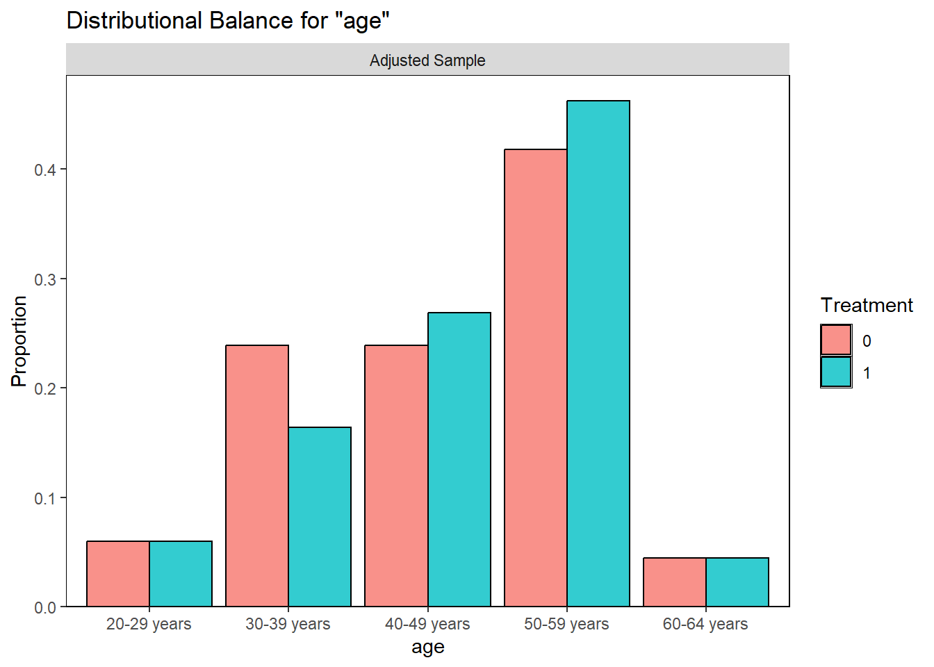
Visually inspect the PS and assess the balance of covariates in the matched sample. Various plots are generated to visualize the distribution of PS across treatment groups and to check the balance of covariates before and after matching.
matchit package
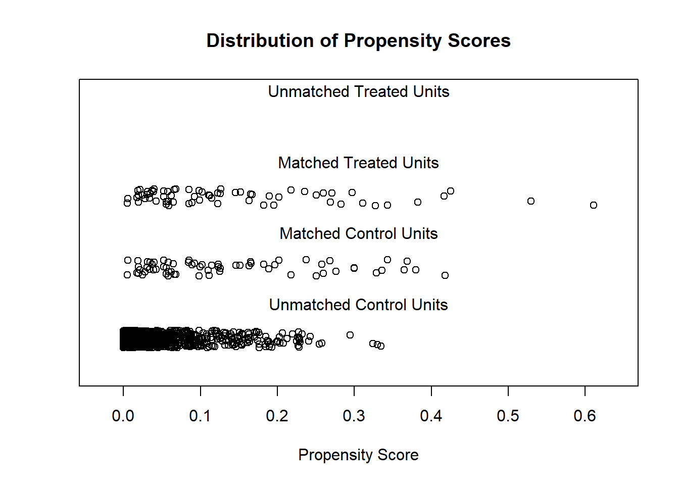
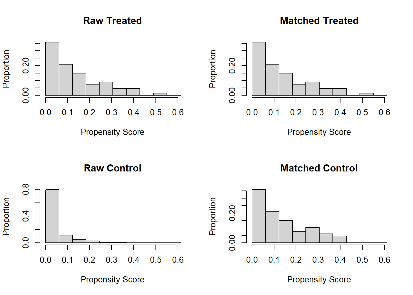

Overalp check
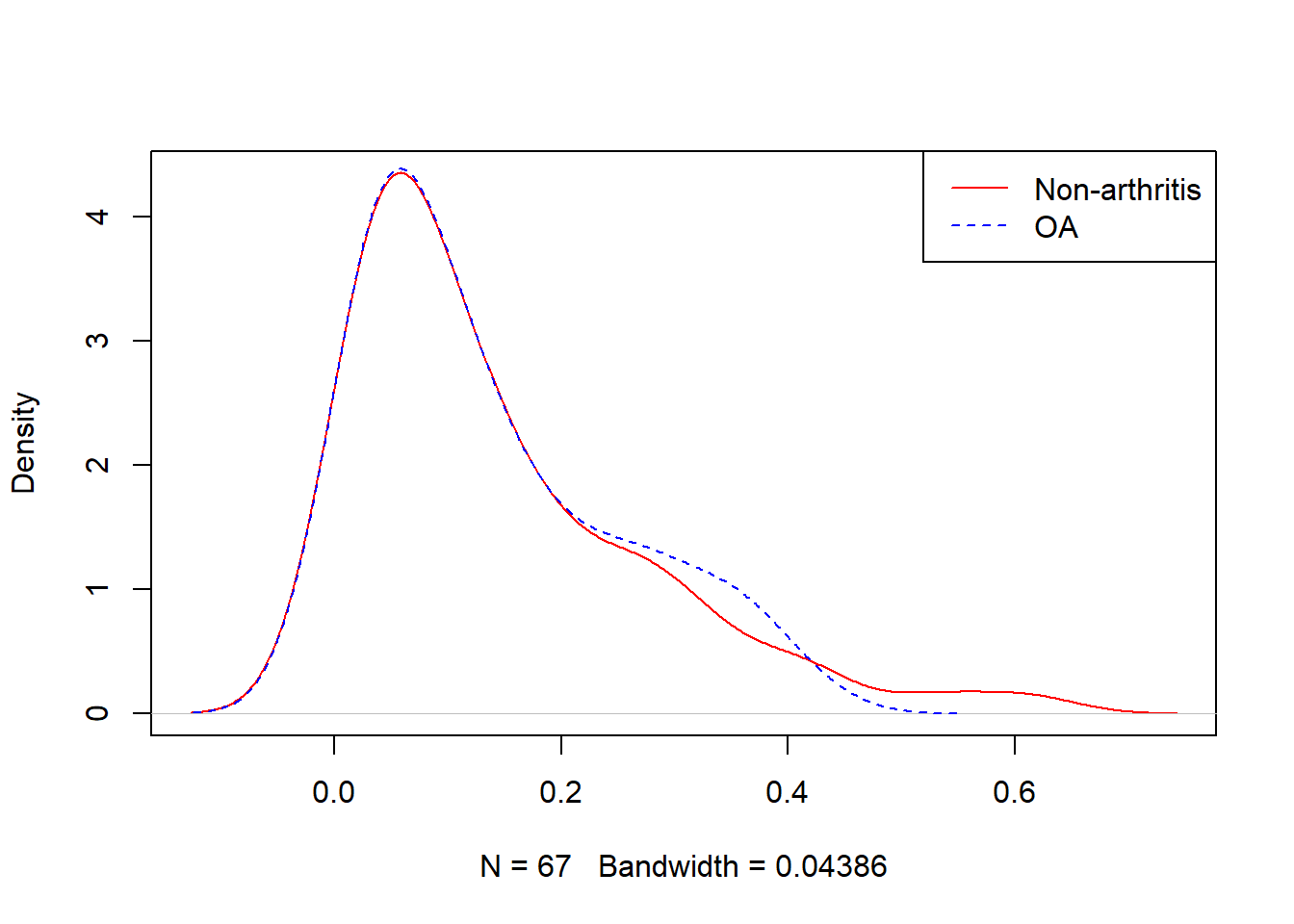
cobalt package
Overlap check in a more convenient way

Look at the data
Numerical values of PS
summary(OACVD.match$distance)
#>     Min.  1st Qu.   Median     Mean  3rd Qu.     Max.
#> 0.004671 0.044834 0.099094 0.138969 0.200576 0.611166
by(OACVD.match$distance, OACVD.match$OA, summary)
#> OACVD.match$OA: 0
#>     Min.  1st Qu.   Median     Mean  3rd Qu.     Max.
#> 0.004671 0.047344 0.099215 0.135042 0.199279 0.418206
#> ------------------------------------------------------------
#> OACVD.match$OA: 1
#>     Min.  1st Qu.   Median     Mean  3rd Qu.     Max.
#> 0.004671 0.047346 0.098973 0.142897 0.198741 0.611166
Question for the students
- Are you happy with the matching after reviewing the plots?
Covariate balance in matched sample
Covariate balance is assessed numerically using standardized mean differences (SMD).
Standardized mean differences: SMD is a versatile and widely used statistical measure that facilitates the comparison of groups in research by providing a scale-free metric of difference and balance. In the context of propensity score matching, achieving low SMD values for covariates after matching is crucial to ensuring the validity of causal inferences drawn from the matched sample.
Benifits:
- SMD is not influenced by the scale of the measured variable, making it suitable for comparing the balance of different variables measured on different scales.
- Unlike hypothesis testing, SMD is not affected by sample size, making it a reliable measure for assessing balance in matched samples.
tab1 <- CreateTableOne(strata = "OA", data = OACVD.match,
test = FALSE, vars = var.names)
print(tab1, smd = TRUE)
#> Stratified by OA
#> 0 1 SMD
#> n 67 67
#> age (%) 0.190
#> 20-29 years 4 ( 6.0) 4 ( 6.0)
#> 30-39 years 16 (23.9) 11 (16.4)
#> 40-49 years 16 (23.9) 18 (26.9)
#> 50-59 years 28 (41.8) 31 (46.3)
#> 60-64 years 3 ( 4.5) 3 ( 4.5)
#> 65 years and over 0 ( 0.0) 0 ( 0.0)
#> teen 0 ( 0.0) 0 ( 0.0)
#> sex = Male (%) 28 (41.8) 32 (47.8) 0.120
#> stress = stressed (%) 20 (29.9) 21 (31.3) 0.032
#> married = single (%) 22 (32.8) 23 (34.3) 0.032
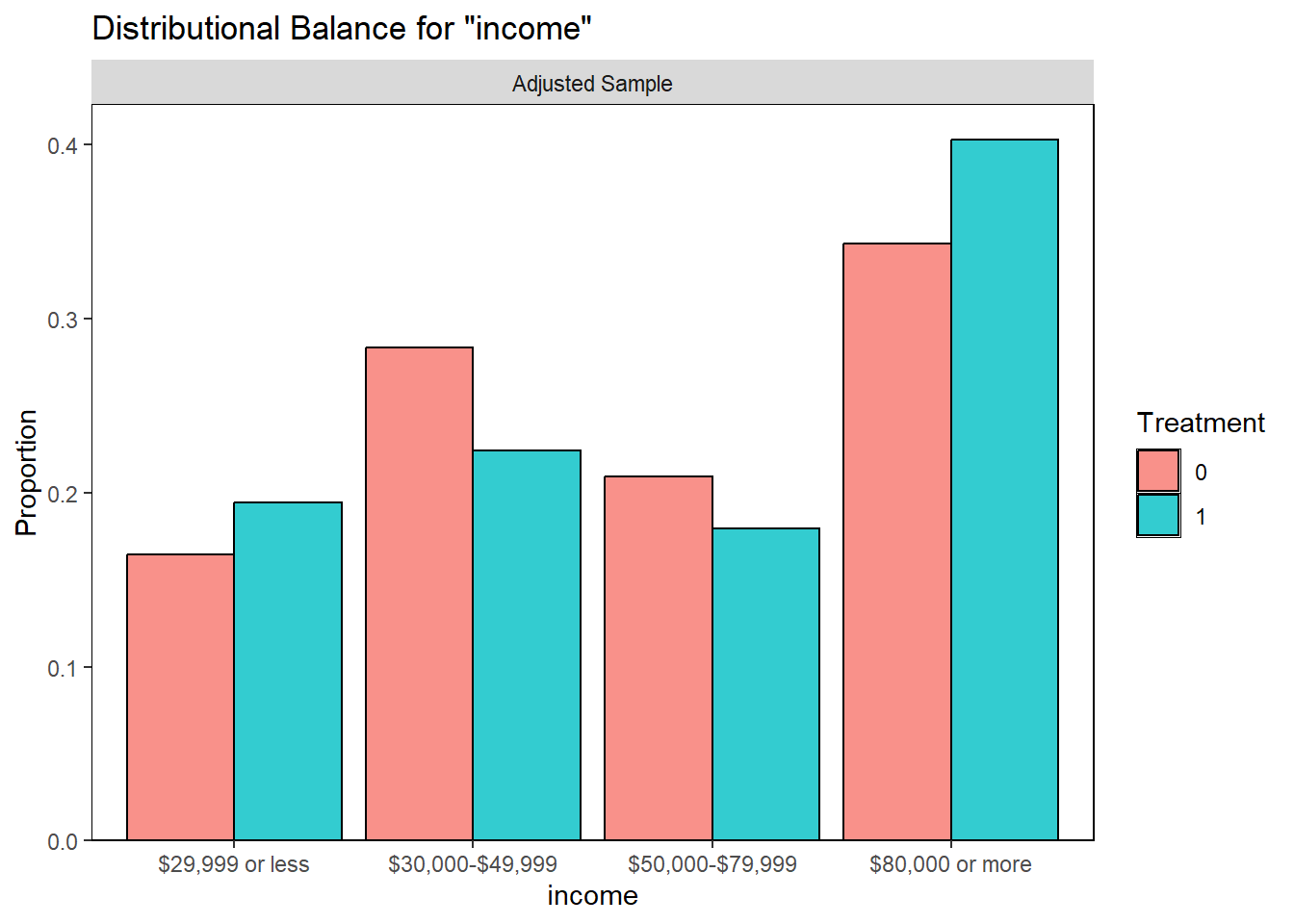
#> income (%) 0.183
#> $29,999 or less 11 (16.4) 13 (19.4)
#> $30,000-$49,999 19 (28.4) 15 (22.4)
#> $50,000-$79,999 14 (20.9) 12 (17.9)
#> $80,000 or more 23 (34.3) 27 (40.3)
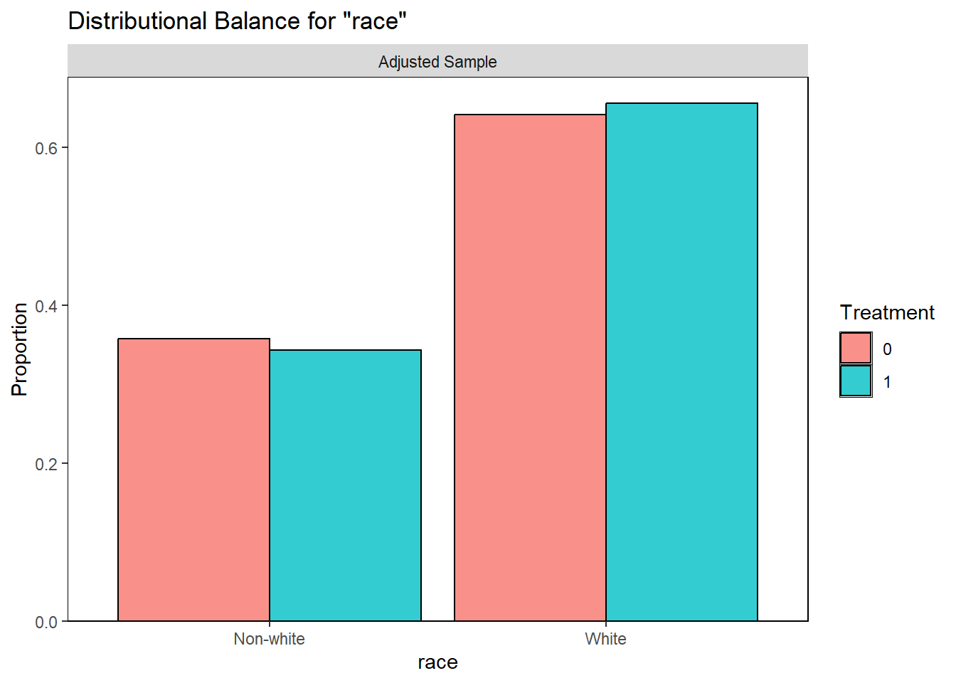
#> race = White (%) 43 (64.2) 44 (65.7) 0.031
#> bmi (%) <0.001
#> Underweight 0 ( 0.0) 0 ( 0.0)
#> healthy weight 18 (26.9) 18 (26.9)
#> Overweight 49 (73.1) 49 (73.1)
#> phyact (%) 0.041
#> Active 16 (23.9) 16 (23.9)
#> Inactive 40 (59.7) 39 (58.2)
#> Moderate 11 (16.4) 12 (17.9)
#> smoke (%) 0.258
#> Never smoker 14 (20.9) 9 (13.4)
#> Current smoker 20 (29.9) 27 (40.3)
#> Former smoker 33 (49.3) 31 (46.3)
#> doctor = Yes (%) 51 (76.1) 47 (70.1) 0.135
#> drink (%) 0.116
#> Never drank 2 ( 3.0) 2 ( 3.0)
#> Current drinker 54 (80.6) 51 (76.1)
#> Former driker 11 (16.4) 14 (20.9)
#> bp = Yes (%) 7 (10.4) 5 ( 7.5) 0.105
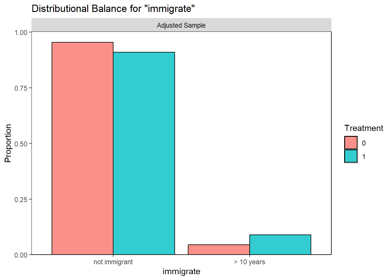
#> immigrate (%) 0.180
#> not immigrant 64 (95.5) 61 (91.0)
#> > 10 years 3 ( 4.5) 6 ( 9.0)
#> recent 0 ( 0.0) 0 ( 0.0)
#> fruit (%) 0.146
#> 0-3 daily serving 19 (28.4) 19 (28.4)
#> 4-6 daily serving 28 (41.8) 32 (47.8)
#> 6+ daily serving 20 (29.9) 16 (23.9)
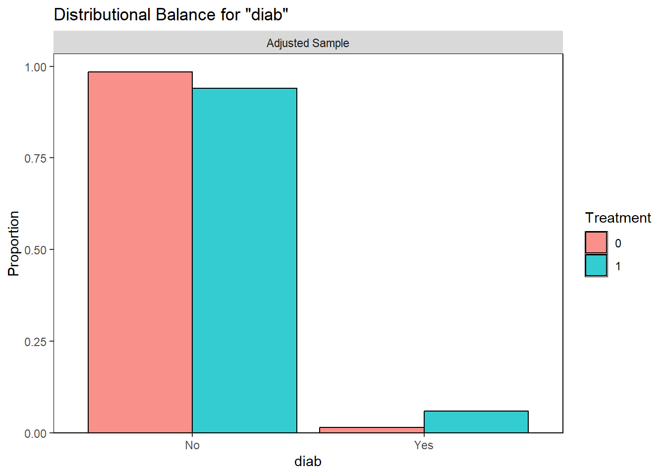
#> diab = Yes (%) 1 ( 1.5) 4 ( 6.0) 0.238
#> edu (%) 0.105
#> < 2ndary 14 (20.9) 13 (19.4)
#> 2nd grad. 1 ( 1.5) 2 ( 3.0)
#> Other 2nd grad. 1 ( 1.5) 1 ( 1.5)
#> Post-2nd grad. 51 (76.1) 51 (76.1)Question for the students
- All SMD < 0.20?
Other balance measures
Individual categories
If you want to check balance at each category (not very useful in general situations). We are generally interested if the variables are balanced or not (not categories).
baltab <- bal.tab(matching.obj)
baltab
#> Balance Measures
#>                             Type Diff.Adj
#> distance                Distance   0.0597
#> age_20-29 years           Binary   0.0000
#> age_30-39 years           Binary  -0.0746
#> age_40-49 years           Binary   0.0299
#> age_50-59 years           Binary   0.0448
#> age_60-64 years           Binary   0.0000
#> sex_Male                  Binary   0.0597
#> stress_stressed           Binary   0.0149
#> married_single            Binary   0.0149
#> income_$29,999 or less    Binary   0.0299
#> income_$30,000-$49,999    Binary  -0.0597
#> income_$50,000-$79,999    Binary  -0.0299
#> income_$80,000 or more    Binary   0.0597
#> race_White                Binary   0.0149
#> bmi_Underweight           Binary   0.0000
#> bmi_healthy weight        Binary   0.0000
#> bmi_Overweight            Binary   0.0000
#> phyact_Active             Binary   0.0000
#> phyact_Inactive           Binary  -0.0149
#> phyact_Moderate           Binary   0.0149
#> smoke_Never smoker        Binary  -0.0746
#> smoke_Current smoker      Binary   0.1045
#> smoke_Former smoker       Binary  -0.0299
#> doctor_Yes                Binary  -0.0597
#> drink_Never drank         Binary   0.0000
#> drink_Current drinker     Binary  -0.0448
#> drink_Former driker       Binary   0.0448
#> bp_Yes                    Binary  -0.0299
#> immigrate_not immigrant   Binary  -0.0448
#> immigrate_> 10 years      Binary   0.0448
#> immigrate_recent          Binary   0.0000
#> fruit_0-3 daily serving   Binary   0.0000
#> fruit_4-6 daily serving   Binary   0.0597
#> fruit_6+ daily serving    Binary  -0.0597
#> diab_Yes                  Binary   0.0448
#> edu_< 2ndary              Binary  -0.0149
#> edu_2nd grad.             Binary   0.0149
#> edu_Other 2nd grad.       Binary   0.0000
#> edu_Post-2nd grad.        Binary   0.0000
#>
#> Sample sizes
#>           Control Treated
#> All          1357      67
#> Matched        67      67
#> Unmatched    1290       0
Individual plots
You could plot each variables individually
Love plot
# Individual categories again
love.plot(baltab, threshold = .2)
#> Warning: Unadjusted values are missing. This can occur when `un = FALSE` and
#> `quick = TRUE` in the original call to `bal.tab()`.
#> Warning: Standardized mean differences and raw mean differences are present in
#> the same plot. Use the `stars` argument to distinguish between them and
#> appropriately label the x-axis. See `?love.plot` for details.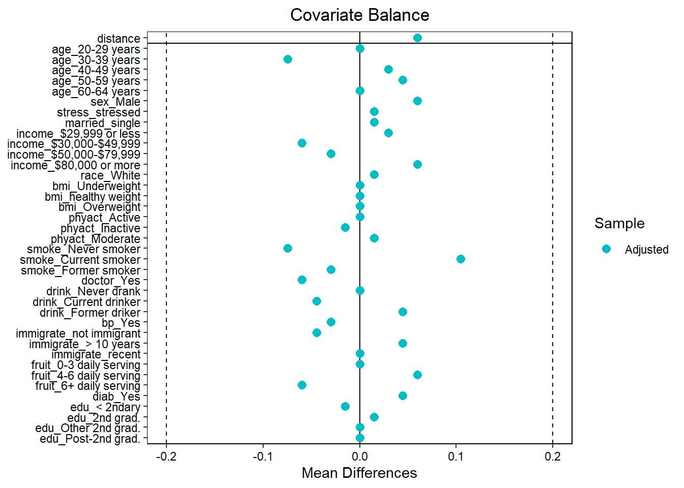
Repeat of Step 1-3 again
Covariate balance is reassessed in each step to ensure the quality of the match.
Add caliper
The matching process is repeated, this time introducing a caliper to ensure that matches are only made within a specified range of PS.
logitPS <-  -log(1/OACVD.match$distance - 1)
# logit of the propensity score
.2*sd(logitPS) # suggested in the literature
#> [1] 0.2334615


# Step 1 and 2
matching.obj <- matchit(ps.formula,
                        data = analytic11n,
                        method = "nearest",
                        ratio = 1,
                        caliper = .2*sd(logitPS))
#> Warning: glm.fit: fitted probabilities numerically 0 or 1 occurred
# see how many matched
matching.obj
#> A `matchit` object
#>  - method: 1:1 nearest neighbor matching without replacement
#>  - distance: Propensity score [caliper]
#>
#>              - estimated with logistic regression
#>  - caliper: <distance> (0.015)
#>  - number of obs.: 1424 (original), 128 (matched)
#>  - target estimand: ATT
#>  - covariates: age, sex, stress, married, income, race, bmi, phyact, smoke, doctor, drink, bp, immigrate, fruit, diab, edu
OACVD.match <- match.data(matching.obj)
# Step 3
by(OACVD.match$distance, OACVD.match$OA, summary)
#> OACVD.match$OA: 0
#> Min. 1st Qu. Median Mean 3rd Qu. Max.
#> 0.004671 0.041740 0.094963 0.124665 0.184103 0.418206
#> ------------------------------------------------------------
#> OACVD.match$OA: 1
#> Min. 1st Qu. Median Mean 3rd Qu. Max.
#> 0.004671 0.041694 0.095089 0.125262 0.183739 0.424895
tab1 <- CreateTableOne(strata = "OA", data = OACVD.match,
test = FALSE, vars = var.names)
print(tab1, smd = TRUE)
#> Stratified by OA
#> 0 1 SMD
#> n 64 64
#> age (%) 0.196
#> 20-29 years 4 ( 6.2) 4 ( 6.2)
#> 30-39 years 16 (25.0) 11 (17.2)
#> 40-49 years 16 (25.0) 18 (28.1)
#> 50-59 years 25 (39.1) 28 (43.8)
#> 60-64 years 3 ( 4.7) 3 ( 4.7)
#> 65 years and over 0 ( 0.0) 0 ( 0.0)
#> teen 0 ( 0.0) 0 ( 0.0)
#> sex = Male (%) 27 (42.2) 30 (46.9) 0.094
#> stress = stressed (%) 18 (28.1) 18 (28.1) <0.001
#> married = single (%) 21 (32.8) 23 (35.9) 0.066
#> income (%) 0.204
#> $29,999 or less 11 (17.2) 13 (20.3)
#> $30,000-$49,999 19 (29.7) 14 (21.9)
#> $50,000-$79,999 13 (20.3) 12 (18.8)
#> $80,000 or more 21 (32.8) 25 (39.1)
#> race = White (%) 40 (62.5) 42 (65.6) 0.065
#> bmi (%) <0.001
#> Underweight 0 ( 0.0) 0 ( 0.0)
#> healthy weight 18 (28.1) 18 (28.1)
#> Overweight 46 (71.9) 46 (71.9)
#> phyact (%) 0.096
#> Active 14 (21.9) 16 (25.0)
#> Inactive 39 (60.9) 36 (56.2)
#> Moderate 11 (17.2) 12 (18.8)
#> smoke (%) 0.267
#> Never smoker 14 (21.9) 9 (14.1)
#> Current smoker 19 (29.7) 26 (40.6)
#> Former smoker 31 (48.4) 29 (45.3)
#> doctor = Yes (%) 48 (75.0) 44 (68.8) 0.139
#> drink (%) 0.123
#> Never drank 2 ( 3.1) 2 ( 3.1)
#> Current drinker 52 (81.2) 49 (76.6)
#> Former driker 10 (15.6) 13 (20.3)
#> bp = Yes (%) 7 (10.9) 5 ( 7.8) 0.107
#> immigrate (%) 0.260
#> not immigrant 62 (96.9) 58 (90.6)
#> > 10 years 2 ( 3.1) 6 ( 9.4)
#> recent 0 ( 0.0) 0 ( 0.0)
#> fruit (%) 0.116
#> 0-3 daily serving 19 (29.7) 19 (29.7)
#> 4-6 daily serving 27 (42.2) 30 (46.9)
#> 6+ daily serving 18 (28.1) 15 (23.4)
#> diab = Yes (%) 0 ( 0.0) 3 ( 4.7) 0.314
#> edu (%) 0.108
#> < 2ndary 14 (21.9) 13 (20.3)
#> 2nd grad. 1 ( 1.6) 2 ( 3.1)
#> Other 2nd grad. 1 ( 1.6) 1 ( 1.6)
#> Post-2nd grad. 48 (75.0) 48 (75.0)Question for the students
- Did all of the SMDs decrease?
Look at the data
Step 4
Estimate treatment effect for matched data
Different models (e.g., unconditional logistic regression, survey design) are fitted to estimate the treatment effect in the matched sample.
Unconditional logistic
Survey design
Convert data to design
The matched data is converted to a survey design object to account for the matched pairs in the analysis.
analytic.miss$matched <- 0
length(analytic.miss$ID) # full data
#> [1] 397173
length(OACVD.match$ID) # matched data
#> [1] 128
length(analytic.miss$ID[analytic.miss$ID %in% OACVD.match$ID])
#> [1] 128
analytic.miss$matched[analytic.miss$ID %in% OACVD.match$ID] <- 1
table(analytic.miss$matched)
#>
#>      0      1
#> 397045    128
w.design0 <- svydesign(id=~1, weights=~survey.weight,
                      data=analytic.miss)
w.design.m <- subset(w.design0, matched == 1)
Balance in matched population?
tab1 <- svyCreateTableOne(strata = "OA", data = w.design.m,
                       test = FALSE, vars = var.names)
print(tab1, smd = TRUE)
#>                        Stratified by OA
#>                         0              1              SMD
#>   n                     1783.6         2002.1
#>   age (%)                                              0.307
#>      20-29 years         131.0 ( 7.3)   120.9 ( 6.0)
#>      30-39 years         388.0 (21.8)   237.8 (11.9)
#>      40-49 years         518.3 (29.1)   572.7 (28.6)
#>      50-59 years         680.1 (38.1)   999.3 (49.9)
#>      60-64 years          66.1 ( 3.7)    71.4 ( 3.6)
#>      65 years and over     0.0 ( 0.0)     0.0 ( 0.0)
#>      teen                  0.0 ( 0.0)     0.0 ( 0.0)
#>   sex = Male (%)         852.4 (47.8)   985.1 (49.2)   0.028
#>   stress = stressed (%)  544.6 (30.5)   531.8 (26.6)   0.088
#>   married = single (%)   419.8 (23.5)   427.5 (21.4)   0.052
#>   income (%)                                           0.222
#>      $29,999 or less     266.6 (14.9)   352.4 (17.6)
#>      $30,000-$49,999     462.8 (25.9)   348.8 (17.4)
#>      $50,000-$79,999     298.6 (16.7)   315.7 (15.8)
#>      $80,000 or more     755.5 (42.4)   985.2 (49.2)
#>   race = White (%)      1129.2 (63.3)  1364.9 (68.2)   0.103
#>   bmi (%)                                              0.045
#>      Underweight           0.0 ( 0.0)     0.0 ( 0.0)
#>      healthy weight      483.3 (27.1)   583.3 (29.1)
#>      Overweight         1300.2 (72.9)  1418.8 (70.9)
#>   phyact (%)                                           0.054
#>      Active              448.0 (25.1)   493.9 (24.7)
#>      Inactive           1075.2 (60.3)  1176.6 (58.8)
#>      Moderate            260.3 (14.6)   331.5 (16.6)
#>   smoke (%)                                            0.288
#>      Never smoker        400.2 (22.4)   265.8 (13.3)
#>      Current smoker      548.8 (30.8)   836.6 (41.8)
#>      Former smoker       834.6 (46.8)   899.6 (44.9)
#>   doctor = Yes (%)      1376.0 (77.1)  1430.1 (71.4)   0.131
#>   drink (%)                                            0.194
#>      Never drank          44.0 ( 2.5)   112.6 ( 5.6)
#>      Current drinker    1464.1 (82.1)  1510.6 (75.5)
#>      Former driker       275.4 (15.4)   378.9 (18.9)
#>   bp = Yes (%)           166.6 ( 9.3)   153.5 ( 7.7)   0.060
#>   immigrate (%)                                        0.235
#>      not immigrant      1694.8 (95.0)  1774.1 (88.6)
#>      > 10 years           88.8 ( 5.0)   228.0 (11.4)
#>      recent                0.0 ( 0.0)     0.0 ( 0.0)
#>   fruit (%)                                            0.293
#>      0-3 daily serving   426.1 (23.9)   480.8 (24.0)
#>      4-6 daily serving   748.1 (41.9)  1082.3 (54.1)
#>      6+ daily serving    609.4 (34.2)   439.0 (21.9)
#>   diab = Yes (%)           0.0 ( 0.0)    83.6 ( 4.2)   0.295
#>   edu (%)                                              0.172
#>      < 2ndary            324.9 (18.2)   342.8 (17.1)
#>      2nd grad.            18.8 ( 1.1)    47.6 ( 2.4)
#>      Other 2nd grad.      15.2 ( 0.9)    52.2 ( 2.6)
#>      Post-2nd grad.     1424.7 (79.9)  1559.4 (77.9)
Outcome analysis
Matched data with increase ratio
The matching process is repeated with a different ratio (e.g., 1:5) to explore how changing the ratio affects the covariate balance and treatment effect estimation.
# Step 1 and 2
matching.obj <- matchit(ps.formula,
                        data = analytic11n,
                        method = "nearest",
                        ratio = 5,
                        caliper = 0.2)
#> Warning: glm.fit: fitted probabilities numerically 0 or 1 occurred
# see how many matched
matching.obj
#> A `matchit` object
#>  - method: 5:1 nearest neighbor matching without replacement
#>  - distance: Propensity score [caliper]
#>
#>              - estimated with logistic regression
#>  - caliper: <distance> (0.013)
#>  - number of obs.: 1424 (original), 349 (matched)
#>  - target estimand: ATT
#>  - covariates: age, sex, stress, married, income, race, bmi, phyact, smoke, doctor, drink, bp, immigrate, fruit, diab, edu
OACVD.match <- match.data(matching.obj)
# Step 3
by(OACVD.match$distance, OACVD.match$OA, summary)
#> OACVD.match$OA: 0
#>     Min.  1st Qu.   Median     Mean  3rd Qu.     Max.
#> 0.004643 0.039181 0.084421 0.101576 0.146403 0.418206
#> ------------------------------------------------------------
#> OACVD.match$OA: 1
#>     Min.  1st Qu.   Median     Mean  3rd Qu.     Max.
#> 0.004671 0.041694 0.095089 0.125262 0.183739 0.424895
tab1 <- CreateTableOne(strata = "OA", data = OACVD.match,
                       test = FALSE, vars = var.names)
print(tab1, smd = TRUE)
#>                        Stratified by OA
#>                         0           1          SMD
#>   n                     285         64
#>   age (%)                                       0.217
#>      20-29 years         24 ( 8.4)   4 ( 6.2)
#>      30-39 years         59 (20.7)  11 (17.2)
#>      40-49 years         94 (33.0)  18 (28.1)
#>      50-59 years         98 (34.4)  28 (43.8)
#>      60-64 years         10 ( 3.5)   3 ( 4.7)
#>      65 years and over    0 ( 0.0)   0 ( 0.0)
#>      teen                 0 ( 0.0)   0 ( 0.0)
#>   sex = Male (%)        132 (46.3)  30 (46.9)   0.011
#>   stress = stressed (%)  81 (28.4)  18 (28.1)   0.007
#>   married = single (%)   91 (31.9)  23 (35.9)   0.085
#>   income (%)                                    0.065
#>      $29,999 or less     64 (22.5)  13 (20.3)
#>      $30,000-$49,999     65 (22.8)  14 (21.9)
#>      $50,000-$79,999     51 (17.9)  12 (18.8)
#>      $80,000 or more    105 (36.8)  25 (39.1)
#>   race = White (%)      169 (59.3)  42 (65.6)   0.131
#>   bmi (%)                                       0.097
#>      Underweight          0 ( 0.0)   0 ( 0.0)
#>      healthy weight      68 (23.9)  18 (28.1)
#>      Overweight         217 (76.1)  46 (71.9)
#>   phyact (%)                                    0.136
#>      Active              57 (20.0)  16 (25.0)
#>      Inactive           178 (62.5)  36 (56.2)
#>      Moderate            50 (17.5)  12 (18.8)
#>   smoke (%)                                     0.097
#>      Never smoker        46 (16.1)   9 (14.1)
#>      Current smoker     123 (43.2)  26 (40.6)
#>      Former smoker      116 (40.7)  29 (45.3)
#>   doctor = Yes (%)      183 (64.2)  44 (68.8)   0.096
#>   drink (%)                                     0.051
#>      Never drank         10 ( 3.5)   2 ( 3.1)
#>      Current drinker    212 (74.4)  49 (76.6)
#>      Former driker       63 (22.1)  13 (20.3)
#>   bp = Yes (%)           22 ( 7.7)   5 ( 7.8)   0.003
#>   immigrate (%)                                 0.100
#>      not immigrant      266 (93.3)  58 (90.6)
#>      > 10 years          19 ( 6.7)   6 ( 9.4)
#>      recent               0 ( 0.0)   0 ( 0.0)
#>   fruit (%)                                     0.149
#>      0-3 daily serving  104 (36.5)  19 (29.7)
#>      4-6 daily serving  124 (43.5)  30 (46.9)
#>      6+ daily serving    57 (20.0)  15 (23.4)
#>   diab = Yes (%)         12 ( 4.2)   3 ( 4.7)   0.023
#>   edu (%)                                       0.137
#>      < 2ndary            67 (23.5)  13 (20.3)
#>      2nd grad.            9 ( 3.2)   2 ( 3.1)
#>      Other 2nd grad.      9 ( 3.2)   1 ( 1.6)
#>      Post-2nd grad.     200 (70.2)  48 (75.0)
Question for the students
- Did all of the SMDs decrease?
Look at the data
Combining matching weights
Different approaches to incorporating weights (e.g., matching weights, survey weights) are explored.
Not incorporating matching weights
analytic.miss$matched <- 0
length(analytic.miss$ID) # full data
#> [1] 397173
length(OACVD.match$ID) # matched data
#> [1] 349
length(analytic.miss$ID[analytic.miss$ID %in% OACVD.match$ID])
#> [1] 349
analytic.miss$matched[analytic.miss$ID %in% OACVD.match$ID] <- 1
table(analytic.miss$matched)
#>
#>      0      1
#> 396824    349
w.design0 <- svydesign(id=~1, weights=~survey.weight,
                      data=analytic.miss)
w.design.m <- subset(w.design0, matched == 1)Incorporating matching weights
analytic.miss$matched <- 0
length(analytic.miss$ID) # full data
#> [1] 397173
length(OACVD.match$ID) # matched data
#> [1] 349
length(analytic.miss$ID[analytic.miss$ID %in% OACVD.match$ID])
#> [1] 349
analytic.miss$matched[analytic.miss$ID %in% OACVD.match$ID] <- 1
table(analytic.miss$matched)
#>
#>      0      1
#> 396824    349
# multiply with matching (ratio) weights with survey weights
analytic.miss$combined.weight <- 0
analytic.miss$combined.weight[analytic.miss$ID %in% OACVD.match$ID] <-
OACVD.match$weights*OACVD.match$survey.weight
w.design0 <- svydesign(id=~1, weights=~combined.weight,
data=analytic.miss)
w.design.m <- subset(w.design0, matched == 1)Matched with replacement
Matching is performed with replacement, allowing control units to be used in more than one match.
# Step 1 and 2
matching.obj <- matchit(ps.formula,
                        data = analytic11n,
                        method = "nearest",
                        ratio = 5,
                        caliper = 0.2,
                        replace = TRUE)
#> Warning: glm.fit: fitted probabilities numerically 0 or 1 occurred
# see how many matched
matching.obj
#> A `matchit` object
#>  - method: 5:1 nearest neighbor matching with replacement
#>  - distance: Propensity score [caliper]
#>
#>              - estimated with logistic regression
#>  - caliper: <distance> (0.013)
#>  - number of obs.: 1424 (original), 308 (matched)
#>  - target estimand: ATT
#>  - covariates: age, sex, stress, married, income, race, bmi, phyact, smoke, doctor, drink, bp, immigrate, fruit, diab, edu
OACVD.match <- match.data(matching.obj)
# Step 3
by(OACVD.match$distance, OACVD.match$OA, summary)
#> OACVD.match$OA: 0
#>     Min.  1st Qu.   Median     Mean  3rd Qu.     Max.
#> 0.004643 0.034244 0.067224 0.100844 0.148958 0.418206
#> ------------------------------------------------------------
#> OACVD.match$OA: 1
#>     Min.  1st Qu.   Median     Mean  3rd Qu.     Max.
#> 0.004671 0.042322 0.097877 0.129743 0.189256 0.424895
tab1 <- CreateTableOne(strata = "OA", data = OACVD.match,
                       test = FALSE, vars = var.names)
print(tab1, smd = TRUE)
#>                        Stratified by OA
#>                         0           1          SMD
#>   n                     243         65
#>   age (%)                                       0.266
#>      20-29 years         22 ( 9.1)   4 ( 6.2)
#>      30-39 years         57 (23.5)  11 (16.9)
#>      40-49 years         74 (30.5)  18 (27.7)
#>      50-59 years         82 (33.7)  29 (44.6)
#>      60-64 years          8 ( 3.3)   3 ( 4.6)
#>      65 years and over    0 ( 0.0)   0 ( 0.0)
#>      teen                 0 ( 0.0)   0 ( 0.0)
#>   sex = Male (%)        113 (46.5)  31 (47.7)   0.024
#>   stress = stressed (%)  67 (27.6)  19 (29.2)   0.037
#>   married = single (%)   75 (30.9)  23 (35.4)   0.096
#>   income (%)                                    0.079
#>      $29,999 or less     53 (21.8)  13 (20.0)
#>      $30,000-$49,999     57 (23.5)  14 (21.5)
#>      $50,000-$79,999     44 (18.1)  12 (18.5)
#>      $80,000 or more     89 (36.6)  26 (40.0)
#>   race = White (%)      146 (60.1)  42 (64.6)   0.094
#>   bmi (%)                                       0.088
#>      Underweight          0 ( 0.0)   0 ( 0.0)
#>      healthy weight      58 (23.9)  18 (27.7)
#>      Overweight         185 (76.1)  47 (72.3)
#>   phyact (%)                                    0.160
#>      Active              45 (18.5)  16 (24.6)
#>      Inactive           155 (63.8)  37 (56.9)
#>      Moderate            43 (17.7)  12 (18.5)
#>   smoke (%)                                     0.095
#>      Never smoker        40 (16.5)   9 (13.8)
#>      Current smoker     101 (41.6)  26 (40.0)
#>      Former smoker      102 (42.0)  30 (46.2)
#>   doctor = Yes (%)      152 (62.6)  45 (69.2)   0.141
#>   drink (%)                                     0.059
#>      Never drank          9 ( 3.7)   2 ( 3.1)
#>      Current drinker    181 (74.5)  50 (76.9)
#>      Former driker       53 (21.8)  13 (20.0)
#>   bp = Yes (%)           19 ( 7.8)   5 ( 7.7)   0.005
#>   immigrate (%)                                 0.115
#>      not immigrant      228 (93.8)  59 (90.8)
#>      > 10 years          15 ( 6.2)   6 ( 9.2)
#>      recent               0 ( 0.0)   0 ( 0.0)
#>   fruit (%)                                     0.147
#>      0-3 daily serving   87 (35.8)  19 (29.2)
#>      4-6 daily serving  109 (44.9)  31 (47.7)
#>      6+ daily serving    47 (19.3)  15 (23.1)
#>   diab = Yes (%)         11 ( 4.5)   3 ( 4.6)   0.004
#>   edu (%)                                       0.175
#>      < 2ndary            58 (23.9)  13 (20.0)
#>      2nd grad.            8 ( 3.3)   2 ( 3.1)
#>      Other 2nd grad.      9 ( 3.7)   1 ( 1.5)
#>      Post-2nd grad.     168 (69.1)  49 (75.4)
Question for the students
- Did all of the SMDs decrease?
Look at the data
Survey design
The matched data is converted into a survey design object, and the treatment effect is estimated while accounting for the complex survey design.
analytic.miss$matched <- 0
length(analytic.miss$ID) # full data
#> [1] 397173
length(OACVD.match$ID) # matched data
#> [1] 308
length(analytic.miss$ID[analytic.miss$ID %in% OACVD.match$ID])
#> [1] 308
analytic.miss$matched[analytic.miss$ID %in% OACVD.match$ID] <- 1
table(analytic.miss$matched)
#>
#>      0      1
#> 396865    308
# multiply with matching (ratio) weights with survey weights
analytic.miss$combined.weight <- 0
analytic.miss$combined.weight[analytic.miss$ID %in% OACVD.match$ID] <-
OACVD.match$weights*OACVD.match$survey.weight
w.design0 <- svydesign(id=~1, weights=~combined.weight,
data=analytic.miss)
w.design.m <- subset(w.design0, matched == 1)Video content (optional)
For those who prefer a video walkthrough, feel free to watch the video below, which offers a description of an earlier version of the above content.