PSM in OA-CVD (US)

Pre-processing

Load data

Load the dataset and inspect its structure and variables.

load(file="Data/propensityscore/NHANES17.RData") 
ls()
#> [1] "analytic"           "analytic.with.miss"

Visualize missing data patterns.

library(dplyr)
#> 
#> Attaching package: 'dplyr'
#> The following objects are masked from 'package:data.table':
#> 
#>     between, first, last
#> The following objects are masked from 'package:stats':
#> 
#>     filter, lag
#> The following objects are masked from 'package:base':
#> 
#>     intersect, setdiff, setequal, union
analytic.with.miss <- dplyr::select(analytic.with.miss, 
                  cholesterol, #outcome
                  gender, age, born, race, education, 
                  married, income, bmi, diabetes, #predictors
                  weight, psu, strata) #survey features

dim(analytic.with.miss)
#> [1] 9254   13
str(analytic.with.miss)
#> 'data.frame':    9254 obs. of  13 variables:
#>  $ cholesterol: 'labelled' int  NA NA 157 148 189 209 176 NA 238 182 ...
#>   ..- attr(*, "label")= chr "Total Cholesterol (mg/dL)"
#>  $ gender     : chr  "Female" "Male" "Female" "Male" ...
#>  $ age        : 'labelled' int  NA NA 66 NA NA 66 75 NA 56 NA ...
#>   ..- attr(*, "label")= chr "Age in years at screening"
#>  $ born       : chr  "Born in 50 US states or Washingt" "Born in 50 US states or Washingt" "Born in 50 US states or Washingt" "Born in 50 US states or Washingt" ...
#>  $ race       : chr  "Other" "White" "Black" "Other" ...
#>  $ education  : chr  NA NA "High.School" NA ...
#>  $ married    : chr  NA NA "Previously.married" NA ...
#>  $ income     : chr  "Over100k" "Over100k" "<25k" NA ...
#>  $ bmi        : 'labelled' num  17.5 15.7 31.7 21.5 18.1 23.7 38.9 NA 21.3 19.7 ...
#>   ..- attr(*, "label")= chr "Body Mass Index (kg/m**2)"
#>  $ diabetes   : chr  "No" "No" "No" "No" ...
#>  $ weight     : 'labelled' num  8540 42567 8338 8723 7065 ...
#>   ..- attr(*, "label")= chr "Full sample 2 year MEC exam weight"
#>  $ psu        : Factor w/ 2 levels "1","2": 2 1 2 2 1 2 1 1 2 2 ...
#>  $ strata     : Factor w/ 15 levels "134","135","136",..: 12 10 12 1 5 5 3 1 1 14 ...
names(analytic.with.miss)
#>  [1] "cholesterol" "gender"      "age"         "born"        "race"       
#>  [6] "education"   "married"     "income"      "bmi"         "diabetes"   
#> [11] "weight"      "psu"         "strata"

library(DataExplorer)
plot_missing(analytic.with.miss)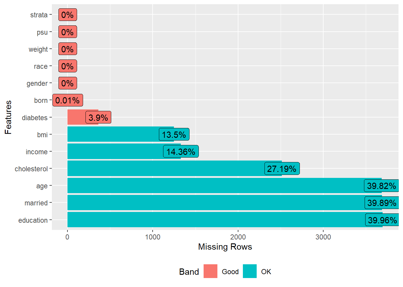

Formatting variables

Rename variables to avoid conflicts. Recode variables into binary or categorical as needed. Ensure variable types (factor, numeric) are appropriate.

# to avaoid any confusion later
# rename weight variable as weights 
# is reserved for matching weights
analytic.with.miss$survey.weight <- analytic.with.miss$weight
analytic.with.miss$weight <- NULL

#Creating binary variable for cholesterol
# Note: 1 = healthy (cholesterol < 200), 0 = unhealthy (cholesterol >= 200)
# This follows the book-wide convention where 1 = healthy.
analytic.with.miss$cholesterol.bin <- ifelse(analytic.with.miss$cholesterol < 200,
                                             1, # healthy
                                             0) # unhealthy
# exposure recoding
analytic.with.miss$diabetes <- ifelse(analytic.with.miss$diabetes == "Yes", 1, 0)

# ID
analytic.with.miss$ID <- 1:nrow(analytic.with.miss)

# covariates
analytic.with.miss$born <- ifelse(analytic.with.miss$born == "Other", 
                                             0,
                                             1)

vars = c("gender", "race", "education", 
         "married", "income", "bmi")

numeric.names <- c("cholesterol", "bmi")
factor.names <- vars[!vars %in% numeric.names] 

analytic.with.miss[factor.names] <- apply(X = analytic.with.miss[factor.names],
                               MARGIN = 2, FUN = as.factor)

analytic.with.miss[numeric.names] <- apply(X = analytic.with.miss[numeric.names],
                                MARGIN = 2, FUN =function (x) 
                                  as.numeric(as.character(x)))
analytic.with.miss$income <- factor(analytic.with.miss$income, 
                                    ordered = TRUE, 
                                levels = c("<25k", "Between.25kto54k", 
                                           "Between.55kto99k", 
                                           "Over100k"))

# features
table(analytic.with.miss$strata)
#> 
#> 134 135 136 137 138 139 140 141 142 143 144 145 146 147 148 
#> 510 638 695 554 605 653 612 693 735 551 689 609 604 596 510
table(analytic.with.miss$psu)
#> 
#>    1    2 
#> 4464 4790
table(analytic.with.miss$strata,analytic.with.miss$psu)
#>      
#>         1   2
#>   134 215 295
#>   135 316 322
#>   136 320 375
#>   137 306 248
#>   138 308 297
#>   139 278 375
#>   140 315 297
#>   141 282 411
#>   142 349 386
#>   143 232 319
#>   144 351 338
#>   145 339 270
#>   146 277 327
#>   147 335 261
#>   148 241 269

# impute
# require(mice)
# imputation1 <- mice(analytic.with.miss, seed = 123,
#                    m = 1, # Number of multiple imputations. 
#                    maxit = 10 # Number of iteration; mostly useful for convergence
#                    )
# analytic.with.miss <- complete(imputation1)
# plot_missing(analytic.with.miss)

Complete case data

Create a dataset (analytic.data) without NA values for analysis. This is done for simplified analysis, but this approach has it’s own challenges. In a next tutorial, we will appropriately deal with missing observations in a propensity score modelling.

dim(analytic.with.miss)
#> [1] 9254   15
analytic.data <- as.data.frame(na.omit(analytic.with.miss))
dim(analytic.data) # complete case
#> [1] 4167   15

Note

Estimand. All three approaches below (Zanutto, DuGoff, Austin) target the same survey-weighted population average treatment effect on the treated (PATT). They differ only in how the survey design enters Steps 1-2 (propensity score estimation and matching), not in the estimand.

Zanutto (2006)

• Ref: Zanutto (2006)

Video content (optional)

Tip

For those who prefer a video walkthrough, feel free to watch the video below, which offers a description of an earlier version of the above content.

Set seed

set.seed(123)

• “it is not necessary to use survey-weighted estimation for the propensity score model”

Propensity score analysis in 4 steps:

• Step 1: PS model specification
• Step 2: Matching based on the estimated propensity scores
• Step 3: Balance checking
• Step 4: Outcome modelling

Step 1

Specify the propensity score model to estimate propensity scores

ps.formula <- as.formula(diabetes ~ gender + born +
                         race + education + married + income + bmi)

Step 2

Match treated and untreated subjects based on the estimated propensity scores. Perform nearest-neighbor matching using the propensity scores. Visualize the distribution of propensity scores before and after matching.

require(MatchIt)
set.seed(123)
# This function fits propensity score model (using logistic 
# regression as above) when specified distance = 'logit'
# performs nearest-neighbor (NN) matching, 
# without replacement 
# with caliper = .2*SD of propensity score  
# within which to draw control units 
# with 1:1 ratio (pair-matching)
match.obj <- matchit(ps.formula, data = analytic.data,
                     distance = 'logit', 
                     method = "nearest", 
                     replace=FALSE,
                     caliper = .2, 
                     ratio = 1)
# see matchit function options here
# https://kosukeimai.github.io/MatchIt/reference/matchit.html
analytic.data$PS <- match.obj$distance
summary(match.obj$distance)
#>    Min. 1st Qu.  Median    Mean 3rd Qu.    Max. 
#> 0.02901 0.12255 0.17658 0.18982 0.23876 0.82164
plot(match.obj, type = "jitter")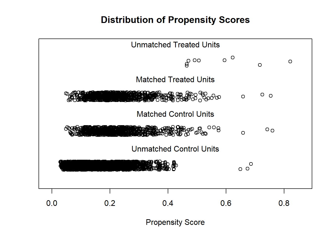

#> To identify the units, use first mouse button; to stop, use second.
plot(match.obj, type = "hist")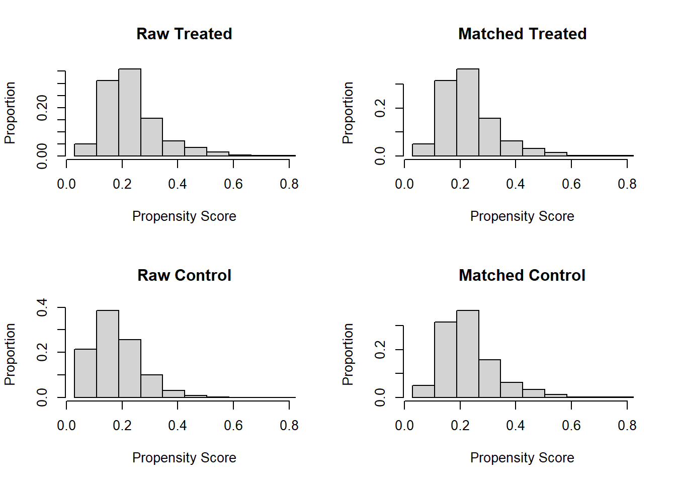

tapply(analytic.data$PS, analytic.data$diabetes, summary)
#> $`0`
#>    Min. 1st Qu.  Median    Mean 3rd Qu.    Max. 
#> 0.02901 0.11509 0.16687 0.17949 0.22816 0.75968 
#> 
#> $`1`
#>    Min. 1st Qu.  Median    Mean 3rd Qu.    Max. 
#> 0.04793 0.16489 0.21300 0.23395 0.27768 0.82164
# check how many matched
match.obj
#> A `matchit` object
#>  - method: 1:1 nearest neighbor matching without replacement
#>  - distance: Propensity score [caliper]
#> 
#>              - estimated with logistic regression
#>  - caliper: <distance> (0.019)
#>  - number of obs.: 4167 (original), 1564 (matched)
#>  - target estimand: ATT
#>  - covariates: gender, born, race, education, married, income, bmi
# extract matched data
matched.data <- match.data(match.obj)

Step 3

Compare the similarity of baseline characteristics between treated and untreated subjects in a the propensity score-matched sample. In this case, we will compare SMD < 0.2 or not.

require(tableone)
baselinevars <- c("gender", "born", "race", "education", 
                  "married", "income", "bmi")
tab1 <- CreateTableOne(strata = "diabetes", vars = baselinevars,
                       data = analytic.data, test = FALSE)
print(tab1, smd = TRUE)
#>                        Stratified by diabetes
#>                         0             1             SMD   
#>   n                      3376           791               
#>   gender = Male (%)      1578 (46.7)    434 (54.9)   0.163
#>   born (mean (SD))       1.00 (0.00)   1.00 (0.00)  <0.001
#>   race (%)                                           0.060
#>      Black                728 (21.6)    183 (23.1)        
#>      Hispanic             727 (21.5)    170 (21.5)        
#>      Other                642 (19.0)    159 (20.1)        
#>      White               1279 (37.9)    279 (35.3)        
#>   education (%)                                      0.185
#>      College             1992 (59.0)    415 (52.5)        
#>      High.School         1174 (34.8)    290 (36.7)        
#>      School               210 ( 6.2)     86 (10.9)        
#>   married (%)                                        0.316
#>      Married             2027 (60.0)    488 (61.7)        
#>      Never.married        631 (18.7)     70 ( 8.8)        
#>      Previously.married   718 (21.3)    233 (29.5)        
#>   income (%)                                         0.092
#>      <25k                 830 (24.6)    225 (28.4)        
#>      Between.25kto54k    1064 (31.5)    244 (30.8)        
#>      Between.55kto99k     778 (23.0)    173 (21.9)        
#>      Over100k             704 (20.9)    149 (18.8)        
#>   bmi (mean (SD))       29.29 (7.11)  32.31 (8.03)   0.399

tab1m <- CreateTableOne(strata = "diabetes", vars = baselinevars, 
                        data = matched.data, test = FALSE)
print(tab1m, smd = TRUE)
#>                        Stratified by diabetes
#>                         0             1             SMD   
#>   n                       782           782               
#>   gender = Male (%)       422 (54.0)    430 (55.0)   0.021
#>   born (mean (SD))       1.00 (0.00)   1.00 (0.00)  <0.001
#>   race (%)                                           0.068
#>      Black                180 (23.0)    179 (22.9)        
#>      Hispanic             151 (19.3)    170 (21.7)        
#>      Other                171 (21.9)    156 (19.9)        
#>      White                280 (35.8)    277 (35.4)        
#>   education (%)                                      0.077
#>      College              441 (56.4)    411 (52.6)        
#>      High.School          262 (33.5)    286 (36.6)        
#>      School                79 (10.1)     85 (10.9)        
#>   married (%)                                        0.044
#>      Married              502 (64.2)    486 (62.1)        
#>      Never.married         63 ( 8.1)     69 ( 8.8)        
#>      Previously.married   217 (27.7)    227 (29.0)        
#>   income (%)                                         0.065
#>      <25k                 202 (25.8)    218 (27.9)        
#>      Between.25kto54k     236 (30.2)    244 (31.2)        
#>      Between.55kto99k     187 (23.9)    171 (21.9)        
#>      Over100k             157 (20.1)    149 (19.1)        
#>   bmi (mean (SD))       32.12 (8.29)  32.05 (7.58)   0.009

Step 4

Estimate the effect of treatment on outcomes using propensity score-matched sample. Use the matched sample to estimate the treatment effect, considering survey design.

Incorporating the survey design into both linear regression and propensity score analysis is crucial. Neglecting the survey weights can significantly impact the estimates, altering the representation of population-level effects.

require(survey)
# setup the design with survey features
analytic.with.miss$matched <- 0
length(analytic.with.miss$ID) # full data
#> [1] 9254
length(matched.data$ID) # matched data
#> [1] 1564
length(analytic.with.miss$ID[analytic.with.miss$ID %in% matched.data$ID])
#> [1] 1564
analytic.with.miss$matched[analytic.with.miss$ID %in% matched.data$ID] <- 1
table(analytic.with.miss$matched)
#> 
#>    0    1 
#> 7690 1564
w.design0 <- svydesign(strata=~strata, id=~psu, weights=~survey.weight, 
                      data=analytic.with.miss, nest=TRUE)
w.design.m <- subset(w.design0, matched == 1)

out.formula <- as.formula(cholesterol.bin ~ diabetes)
sfit <- svyglm(out.formula,family=binomial(logit), design = w.design.m)
#> Warning in eval(family$initialize): non-integer #successes in a binomial glm!
require(jtools)
summ(sfit, exp = TRUE, confint = TRUE)

Observations	1564
Dependent variable	cholesterol.bin
Type	Survey-weighted generalized linear model
Family	binomial
Link	logit

Pseudo-R² (Cragg-Uhler)	0.02
Pseudo-R² (McFadden)	0.01
AIC	1925.24

	exp(Est.)	2.5%	97.5%	t val.	p
(Intercept)	1.33	0.97	1.80	1.79	0.09
diabetes	1.68	1.17	2.41	2.84	0.01
Standard errors: Robust

Important

Interpreting the outcome model. Here the outcome cholesterol.bin is coded so that 1 = healthy (cholesterol < 200) and 0 = unhealthy. A binomial glm/svyglm models the probability of the non-reference level, so this model estimates P(healthy). The odds ratio for diabetes therefore describes the odds of being healthy (desirable cholesterol): an OR < 1 means diabetes is associated with lower odds of healthy cholesterol. This event direction (event = healthy) applies to all of the outcome models in this tutorial and follows the book-wide 1 = healthy coding convention.

All outcome models in this tutorial use family = binomial (the convention used throughout this module). Because the standard errors here come from the survey design, the choice between binomial and quasibinomial does not affect the reported svyglm standard errors; binomial may emit a non-integer-successes warning when survey weights are non-integer, but the inference is unchanged.

DuGoff et al. (2014)

• Ref: DuGoff, Schuler, and Stuart (2014)

Propensity score analysis in 4 steps

Video content (optional)

Tip

For those who prefer a video walkthrough, feel free to watch the video below, which offers a description of an earlier version of the above content.

Step 1

Specify the propensity score model to estimate propensity scores. Similar to Zanutto but includes additional covariates in the model.

# response = exposure variable
# independent variables = baseline covariates
ps.formula <- as.formula(diabetes ~ gender + born + race + education + 
                            married + income + bmi+
                           psu+strata+survey.weight)

Step 2

Match treated and untreated subjects on the estimated propensity scores

require(MatchIt)
set.seed(123)
match.obj <- matchit(ps.formula, data = analytic.data,
                     distance = 'logit', 
                     method = "nearest", 
                     replace=FALSE,
                     caliper = .2, 
                     ratio = 1)
analytic.data$PS <- match.obj$distance
summary(match.obj$distance)
#>    Min. 1st Qu.  Median    Mean 3rd Qu.    Max. 
#> 0.00363 0.11341 0.17509 0.18982 0.24766 0.80853
plot(match.obj, type = "jitter")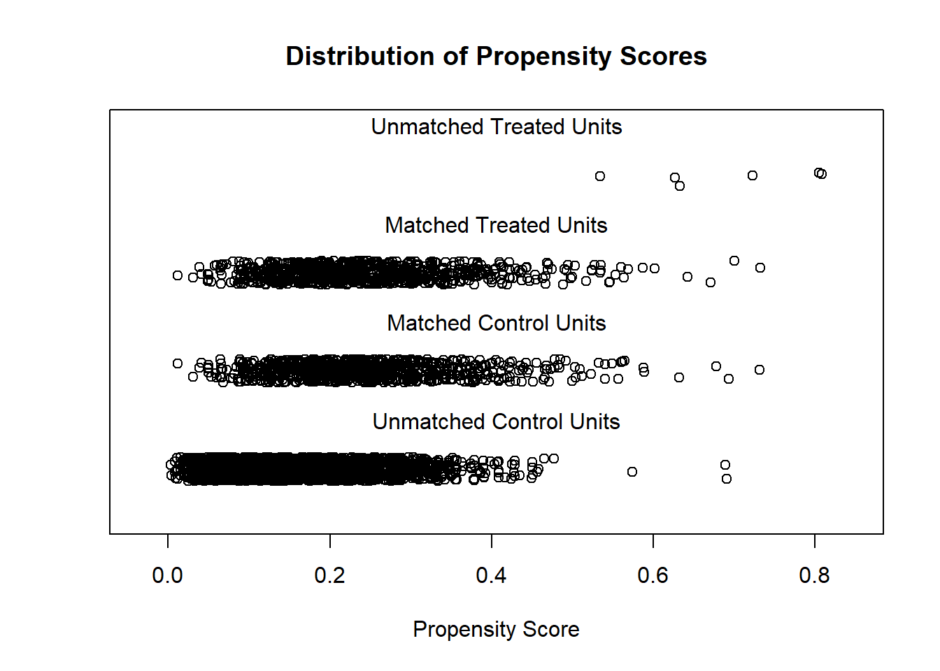

#> To identify the units, use first mouse button; to stop, use second.
plot(match.obj, type = "hist")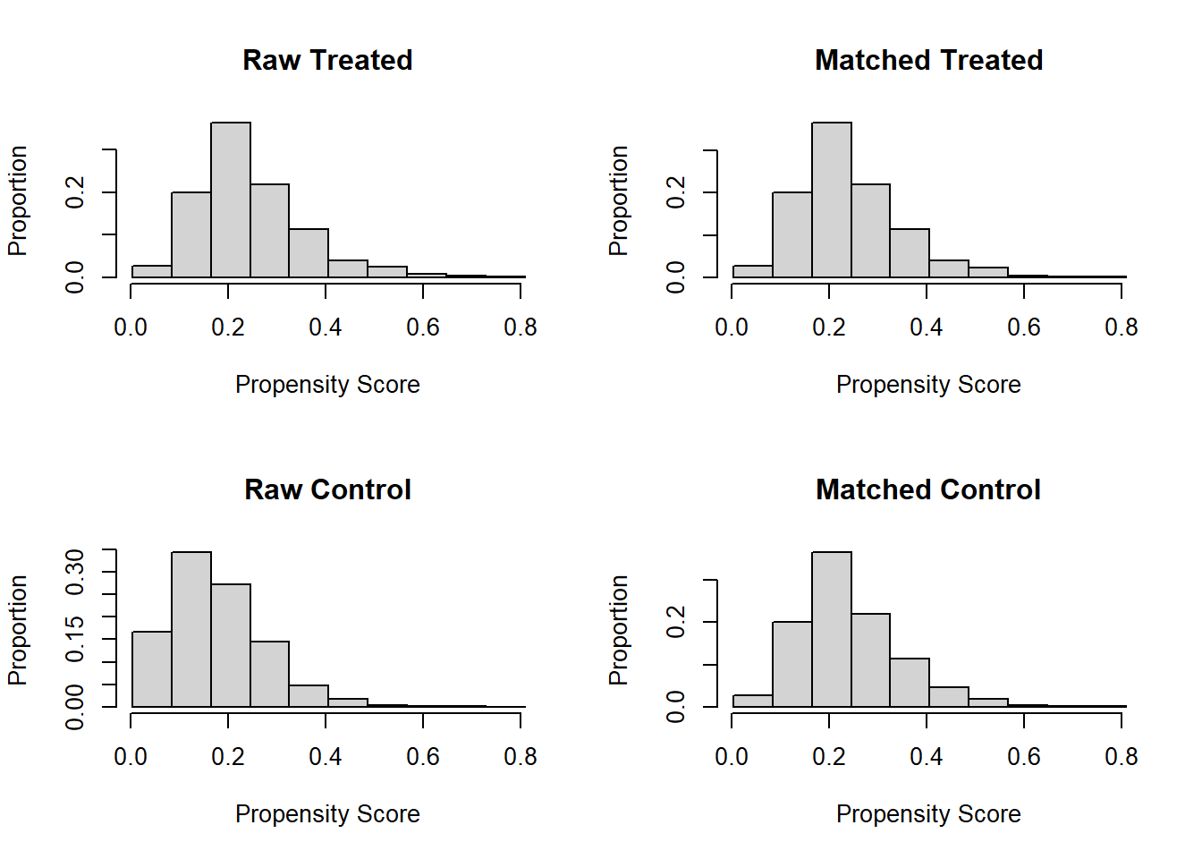

tapply(analytic.data$PS, analytic.data$diabetes, summary)
#> $`0`
#>    Min. 1st Qu.  Median    Mean 3rd Qu.    Max. 
#> 0.00363 0.10394 0.16243 0.17690 0.23461 0.73143 
#> 
#> $`1`
#>    Min. 1st Qu.  Median    Mean 3rd Qu.    Max. 
#> 0.01182 0.17245 0.22748 0.24500 0.29948 0.80853
# check how many matched
match.obj
#> A `matchit` object
#>  - method: 1:1 nearest neighbor matching without replacement
#>  - distance: Propensity score [caliper]
#> 
#>              - estimated with logistic regression
#>  - caliper: <distance> (0.021)
#>  - number of obs.: 4167 (original), 1570 (matched)
#>  - target estimand: ATT
#>  - covariates: gender, born, race, education, married, income, bmi, psu, strata, survey.weight
# extract matched data
matched.data <- match.data(match.obj)

Step 3

Compare the similarity of baseline characteristics between treated and untreated subjects in a the propensity score-matched sample. In this case, we will compare SMD < 0.2 or not.

require(tableone)
baselinevars <- c("gender", "born", "race", "education", 
                  "married", "income", "bmi", 
                  "psu", "strata", "survey.weight")
matched.data$survey.weight <- as.numeric(as.character(matched.data$survey.weight))
matched.data$strata <- as.numeric(as.character(matched.data$strata))
tab1m <- CreateTableOne(strata = "diabetes", vars = baselinevars,
                        data = matched.data, test = FALSE)
print(tab1m, smd = TRUE)
#>                            Stratified by diabetes
#>                             0                   1                   SMD   
#>   n                              785                 785                  
#>   gender = Male (%)              433 (55.2)          431 (54.9)      0.005
#>   born (mean (SD))              1.00 (0.00)         1.00 (0.00)     <0.001
#>   race (%)                                                           0.048
#>      Black                       193 (24.6)          180 (22.9)           
#>      Hispanic                    163 (20.8)          170 (21.7)           
#>      Other                       163 (20.8)          158 (20.1)           
#>      White                       266 (33.9)          277 (35.3)           
#>   education (%)                                                      0.032
#>      College                     403 (51.3)          412 (52.5)           
#>      High.School                 300 (38.2)          288 (36.7)           
#>      School                       82 (10.4)           85 (10.8)           
#>   married (%)                                                        0.030
#>      Married                     473 (60.3)          484 (61.7)           
#>      Never.married                71 ( 9.0)           70 ( 8.9)           
#>      Previously.married          241 (30.7)          231 (29.4)           
#>   income (%)                                                         0.035
#>      <25k                        232 (29.6)          222 (28.3)           
#>      Between.25kto54k            236 (30.1)          242 (30.8)           
#>      Between.55kto99k            176 (22.4)          173 (22.0)           
#>      Over100k                    141 (18.0)          148 (18.9)           
#>   bmi (mean (SD))              31.92 (8.33)        32.09 (7.52)      0.020
#>   psu = 2 (%)                    382 (48.7)          394 (50.2)      0.031
#>   strata (mean (SD))          140.84 (4.24)       140.97 (4.23)      0.031
#>   survey.weight (mean (SD)) 35647.01 (37699.98) 35596.81 (45212.82)  0.001

Note that here the design variables (psu, strata, survey.weight) are reported with the same SMD < 0.2 balance criterion as the confounders. Their interpretive role differs, however: balancing the design variables is part of the DuGoff strategy for incorporating the survey design into the propensity score, whereas balancing the confounders is what removes confounding bias in the matched sample.

Step 4

Estimate the effect of treatment on outcomes using propensity score-matched sample

# setup the design with survey features
analytic.with.miss$matched <- 0
length(analytic.with.miss$ID) # full data
#> [1] 9254
length(matched.data$ID) # matched data
#> [1] 1570
length(analytic.with.miss$ID[analytic.with.miss$ID %in% matched.data$ID])
#> [1] 1570
analytic.with.miss$matched[analytic.with.miss$ID %in% matched.data$ID] <- 1
table(analytic.with.miss$matched)
#> 
#>    0    1 
#> 7684 1570
w.design0 <- svydesign(strata=~strata, id=~psu, weights=~survey.weight, 
                      data=analytic.with.miss, nest=TRUE)
w.design.m <- subset(w.design0, matched == 1)

out.formula <- as.formula(cholesterol.bin ~ diabetes)
sfit <- svyglm(out.formula,family=binomial, design = w.design.m)
#> Warning in eval(family$initialize): non-integer #successes in a binomial glm!
require(jtools)
summ(sfit, exp = TRUE, confint = TRUE)

Observations	1570
Dependent variable	cholesterol.bin
Type	Survey-weighted generalized linear model
Family	binomial
Link	logit

Pseudo-R² (Cragg-Uhler)	0.01
Pseudo-R² (McFadden)	0.00
AIC	1918.09

	exp(Est.)	2.5%	97.5%	t val.	p
(Intercept)	1.69	1.33	2.15	4.24	0.00
diabetes	1.32	0.99	1.77	1.86	0.08
Standard errors: Robust

Austin et al. (2018)

• Ref: Austin, Jembere, and Chiu (2018)

Propensity score analysis in 4 steps

Video content (optional)

Tip

For those who prefer a video walkthrough, feel free to watch the video below, which offers a description of an earlier version of the above content.

Step 1

Specify the propensity score model to estimate propensity scores. Use survey logistic regression to account for survey design in propensity score estimation.

# response = exposure variable
# independent variables = baseline covariates
ps.formula <- as.formula(diabetes ~ gender + born + race + education + 
                            married + income + bmi)
require(survey)
analytic.design <- svydesign(id=~psu,weights=~survey.weight, 
                             strata=~strata,
                             data=analytic.data, nest=TRUE)
ps.fit <- svyglm(ps.formula, design=analytic.design, family=quasibinomial)
analytic.data$PS <- fitted(ps.fit)
summary(analytic.data$PS)
#>    Min. 1st Qu.  Median    Mean 3rd Qu.    Max. 
#> 0.01352 0.08788 0.13399 0.15120 0.19285 0.86375

Step 2

Match treated and untreated subjects on the estimated propensity scores. The matched data used downstream (Steps 3-4) come from the MatchIt block below. The Matching package block is shown only as an optional alternative matcher; its result is stored in a separate object (matched.data2.Match) and is not used downstream.

# Optional alternative matcher (Matching package); not used downstream
require(Matching)
match.obj2 <- Match(Y=analytic.data$cholesterol,
                    Tr=analytic.data$diabetes,
                    X=analytic.data$PS,
                    M=1,
                    estimand = "ATT",
                    replace=FALSE,
                    caliper = 0.2)
summary(match.obj2)
#> 
#> Estimate...  -15.287 
#> SE.........  2.118 
#> T-stat.....  -7.2175 
#> p.val......  5.2958e-13 
#> 
#> Original number of observations..............  4167 
#> Original number of treated obs...............  791 
#> Matched number of observations...............  781 
#> Matched number of observations  (unweighted).  781 
#> 
#> Caliper (SDs)........................................   0.2 
#> Number of obs dropped by 'exact' or 'caliper'  10
matched.data2.Match <- analytic.data[c(match.obj2$index.treated,
                                 match.obj2$index.control),]
dim(matched.data2.Match)
#> [1] 1562   16

require(MatchIt)
set.seed(123)
match.obj <- matchit(ps.formula, data = analytic.data,
                     distance = analytic.data$PS, 
                     method = "nearest", 
                     replace=FALSE,
                     caliper = .2, 
                     ratio = 1)
analytic.data$PS <- match.obj$distance
summary(match.obj$distance)
#>    Min. 1st Qu.  Median    Mean 3rd Qu.    Max. 
#> 0.01352 0.08788 0.13399 0.15120 0.19285 0.86375
plot(match.obj, type = "jitter")

#> To identify the units, use first mouse button; to stop, use second.
plot(match.obj, type = "hist")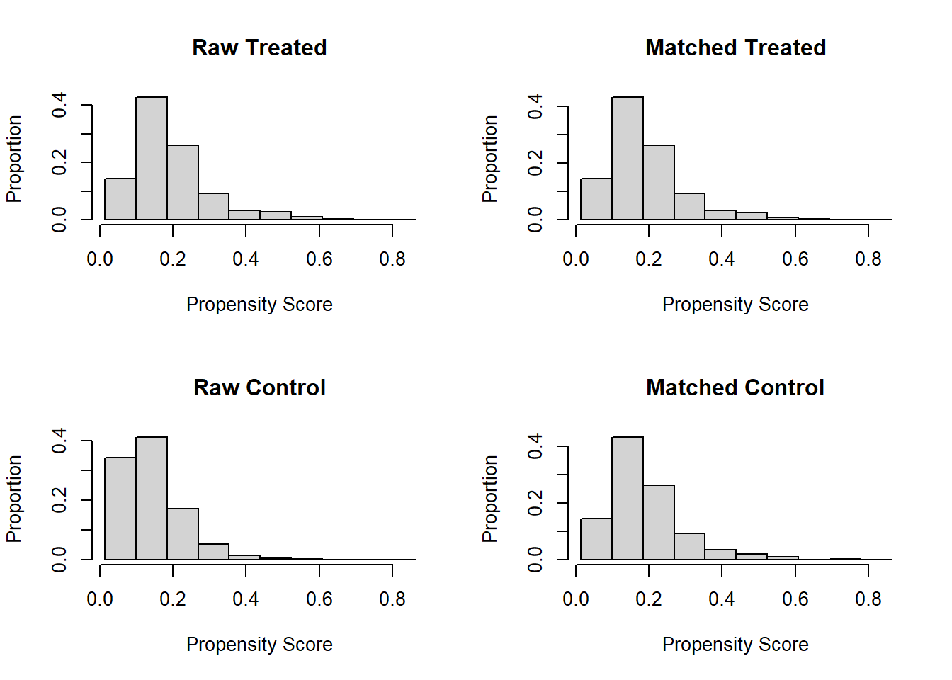

tapply(analytic.data$PS, analytic.data$diabetes, summary)
#> $`0`
#>    Min. 1st Qu.  Median    Mean 3rd Qu.    Max. 
#> 0.01352 0.08182 0.12644 0.14119 0.18267 0.75047 
#> 
#> $`1`
#>    Min. 1st Qu.  Median    Mean 3rd Qu.    Max. 
#> 0.02352 0.12362 0.16998 0.19389 0.23171 0.86375
# check how many matched
match.obj
#> A `matchit` object
#>  - method: 1:1 nearest neighbor matching without replacement
#>  - distance: User-defined [caliper]
#>  - caliper: <distance> (0.019)
#>  - number of obs.: 4167 (original), 1568 (matched)
#>  - target estimand: ATT
#>  - covariates: gender, born, race, education, married, income, bmi
# extract matched data
matched.data2 <- match.data(match.obj)
dim(matched.data2)
#> [1] 1568   19

Step 3

Compare the similarity of baseline characteristics between treated and untreated subjects in a the propensity score-matched sample. In this case, we will compare SMD < 0.2 or not.

baselinevars <- c("gender", "born", "race", "education", 
                  "married", "income", "bmi")
tab1m <- CreateTableOne(strata = "diabetes", 
                           vars = baselinevars,
                           data = matched.data2, test = FALSE)
print(tab1m, smd = TRUE)
#>                        Stratified by diabetes
#>                         0             1             SMD   
#>   n                       784           784               
#>   gender = Male (%)       405 (51.7)    431 (55.0)   0.067
#>   born (mean (SD))       1.00 (0.00)   1.00 (0.00)  <0.001
#>   race (%)                                           0.134
#>      Black                163 (20.8)    182 (23.2)        
#>      Hispanic             139 (17.7)    170 (21.7)        
#>      Other                171 (21.8)    157 (20.0)        
#>      White                311 (39.7)    275 (35.1)        
#>   education (%)                                      0.040
#>      College              428 (54.6)    413 (52.7)        
#>      High.School          274 (34.9)    288 (36.7)        
#>      School                82 (10.5)     83 (10.6)        
#>   married (%)                                        0.070
#>      Married              509 (64.9)    485 (61.9)        
#>      Never.married         59 ( 7.5)     70 ( 8.9)        
#>      Previously.married   216 (27.6)    229 (29.2)        
#>   income (%)                                         0.063
#>      <25k                 220 (28.1)    220 (28.1)        
#>      Between.25kto54k     226 (28.8)    242 (30.9)        
#>      Between.55kto99k     192 (24.5)    173 (22.1)        
#>      Over100k             146 (18.6)    149 (19.0)        
#>   bmi (mean (SD))       31.93 (8.16)  32.11 (7.61)   0.023

Step 4

Estimate the effect of treatment on outcomes using propensity score-matched sample.

# setup the design with survey features
analytic.with.miss$matched <- 0
length(analytic.with.miss$ID) # full data
#> [1] 9254
length(matched.data2$ID) # matched data
#> [1] 1568
length(analytic.with.miss$ID[analytic.with.miss$ID %in% matched.data2$ID])
#> [1] 1568
analytic.with.miss$matched[analytic.with.miss$ID %in% matched.data2$ID] <- 1
table(analytic.with.miss$matched)
#> 
#>    0    1 
#> 7686 1568
w.design0 <- svydesign(strata=~strata, id=~psu, weights=~survey.weight, 
                      data=analytic.with.miss, nest=TRUE)
w.design.m2 <- subset(w.design0, matched == 1)

out.formula <- as.formula(cholesterol.bin ~ diabetes)
sfit <- svyglm(out.formula,family=binomial, design = w.design.m2)
#> Warning in eval(family$initialize): non-integer #successes in a binomial glm!

require(jtools)
summ(sfit, exp = TRUE, confint = TRUE)

Observations	1568
Dependent variable	cholesterol.bin
Type	Survey-weighted generalized linear model
Family	binomial
Link	logit

Pseudo-R² (Cragg-Uhler)	0.01
Pseudo-R² (McFadden)	0.01
AIC	1919.53

	exp(Est.)	2.5%	97.5%	t val.	p
(Intercept)	1.46	1.15	1.86	3.11	0.01
diabetes	1.52	1.21	1.90	3.65	0.00
Standard errors: Robust

Austin, Peter C, Nathaniel Jembere, and Maria Chiu. 2018. “Propensity Score Matching and Complex Surveys.” Statistical Methods in Medical Research 27 (4): 1240–57.

DuGoff, Eva H, Megan Schuler, and Elizabeth A Stuart. 2014. “Generalizing Observational Study Results: Applying Propensity Score Methods to Complex Surveys.” Health Services Research 49 (1): 284–303.

Zanutto, Elaine L. 2006. “A Comparison of Propensity Score and Linear Regression Analysis of Complex Survey Data.” Journal of Data Science 4 (1): 67–91.