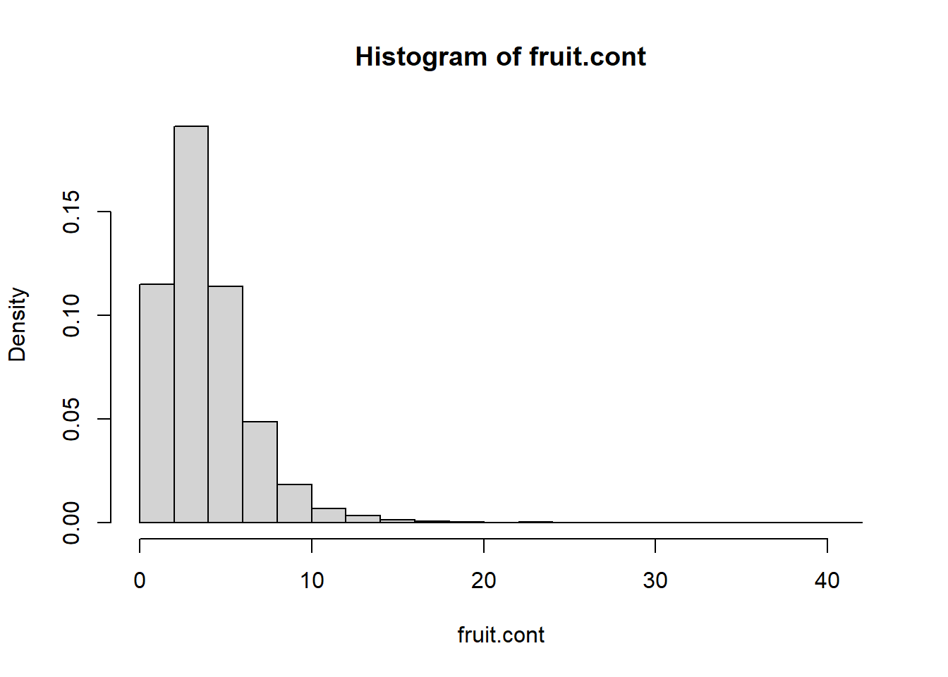
In this tutorial, we will see how to use Poisson and negative binomial regression. In practice, we use Poisson regression to model a count outcome. Note that we assume the mean is equal to the variance in Poisson. When the variance is greater than what’s assumed by the model, overdispersion occurs. Poisson regression of overdispersed data leads to under-estimated or deflated standard errors, which leads to inflated test statistics and overly small (anti-conservative) p-values, increasing false positives. We can use negative binomial regression to model overdispersed data.
# Design-adjusted Poisson - adjusted for covariatesfit2<-svyglm(fruit.cont ~phyact2 + age + sex + income + race + bmicat + smoke + edu, design=w.design, family=poisson)summ(fit2, confint =TRUE, digits =3, vifs =TRUE)
Observations
21623
Dependent variable
fruit.cont
Type
Survey-weighted generalized linear model
Family
poisson
Link
log
Pseudo-R² (Cragg-Uhler)
0.137
Pseudo-R² (McFadden)
0.076
AIC
97795.011
Est.
2.5%
97.5%
t val.
p
VIF
(Intercept)
1.175
1.113
1.237
37.230
0.000
NA
phyact2Active
0.241
0.210
0.272
15.211
0.000
1.346
phyact2Moderate
0.105
0.074
0.135
6.775
0.000
1.346
age40-49 years
0.041
0.010
0.071
2.623
0.009
1.447
age50-59 years
0.102
0.071
0.133
6.402
0.000
1.447
age60-64 years
0.149
0.096
0.203
5.461
0.000
1.447
sexMale
-0.136
-0.161
-0.111
-10.500
0.000
1.148
income$30,000-$49,999
0.025
-0.015
0.066
1.217
0.224
1.294
income$50,000-$79,999
0.031
-0.008
0.070
1.559
0.119
1.294
income$80,000 or more
0.057
0.018
0.096
2.874
0.004
1.294
raceWhite
0.023
-0.012
0.059
1.289
0.197
1.193
bmicatOverweight
-0.009
-0.035
0.017
-0.708
0.479
1.331
bmicatUnderweight
0.029
-0.033
0.091
0.928
0.353
1.331
smokeFormer smoker
0.094
0.059
0.128
5.352
0.000
1.474
smokeNever smoker
0.140
0.102
0.177
7.290
0.000
1.474
edu2nd grad.
0.026
-0.020
0.072
1.093
0.274
1.302
eduOther 2nd grad.
0.033
-0.024
0.090
1.136
0.256
1.302
eduPost-2nd grad.
0.129
0.085
0.173
5.807
0.000
1.302
Standard errors: Robust
Negative binomial regression
Let’s fit the negative binomial regression model using the MASS::glm.nb function, which estimates the dispersion parameter (theta, \(\theta\)) from the data rather than fixing it. In the negative binomial model the variance is \(\text{Var}(Y) = \mu + \mu^2/\theta\), so the variance exceeds the mean whenever \(\theta\) is finite, allowing the model to accommodate overdispersion. As \(\theta \to \infty\) the variance approaches \(\mu\) and the model reduces to Poisson. We report the estimated \(\theta\) alongside the rate ratios.
require(MASS)analytic2$phyact2=relevel(analytic2$phyact, ref ="Inactive")# Negative binomial regression - crudefit3<-glm.nb(fruit.cont ~ phyact2, data=analytic2)fit3$theta # estimated dispersion parameter (theta)#> [1] 10.27349round(exp(cbind(coef(fit3), confint(fit3))),2)#> Waiting for profiling to be done...#> 2.5 % 97.5 %#> (Intercept) 3.81 3.77 3.85#> phyact2Active 1.32 1.29 1.34#> phyact2Moderate 1.15 1.12 1.17# Negative binomial regression - adjusted for covariatesfit4<-glm.nb(fruit.cont ~phyact2 + age + sex + income + race + bmicat + smoke + edu, data=analytic2)fit4$theta # estimated dispersion parameter (theta)#> [1] 12.53347round(exp(cbind(coef(fit4), confint(fit4))),2)#> Waiting for profiling to be done...#> 2.5 % 97.5 %#> (Intercept) 3.18 3.06 3.30#> phyact2Active 1.29 1.26 1.31#> phyact2Moderate 1.12 1.10 1.14#> age40-49 years 1.03 1.01 1.05#> age50-59 years 1.09 1.06 1.11#> age60-64 years 1.14 1.10 1.17#> sexMale 0.84 0.83 0.85#> income$30,000-$49,999 1.04 1.02 1.07#> income$50,000-$79,999 1.05 1.03 1.08#> income$80,000 or more 1.09 1.06 1.11#> raceWhite 1.00 0.97 1.02#> bmicatOverweight 0.98 0.96 0.99#> bmicatUnderweight 1.00 0.96 1.04#> smokeFormer smoker 1.14 1.12 1.16#> smokeNever smoker 1.20 1.17 1.22#> edu2nd grad. 1.04 1.01 1.07#> eduOther 2nd grad. 1.05 1.01 1.09#> eduPost-2nd grad. 1.13 1.10 1.16
The exponentiated coefficients are rate ratios (IRRs). For example, the phyact2 rate ratio compares the expected fruit consumption count for the corresponding physical-activity level relative to the inactive reference group, holding other covariates fixed.
Survey weighted negative binomial regression
Now, let’s fit the design-adjusted negative binomial regression model. The svyglm.nb fit returns the estimated dispersion parameter (theta) together with the mean-model coefficients (prefixed with eta.). We report theta separately and exponentiate only the mean-model (eta.) coefficients to obtain rate ratios; the theta.(Intercept) row is not a rate ratio and should not be exponentiated.
require(sjstats)# Helper: exponentiate only the mean-model (eta.) coefficients as rate ratiosnb_irr <-function(fit){ est <-cbind(coef(fit), confint(fit)) eta.rows <-grepl("^eta\\.", rownames(est))round(exp(est[eta.rows, , drop =FALSE]), 2)}# Design-adjusted negative binomial - crudefit3<-svyglm.nb(fruit.cont ~phyact2, design=w.design)attr(fit3, "nb.theta") # estimated dispersion parameter (theta)#> [1] 10.27019nb_irr(fit3)#> 2.5 % 97.5 %#> eta.(Intercept) 3.95 3.87 4.02#> eta.phyact2Active 1.30 1.26 1.34#> eta.phyact2Moderate 1.13 1.10 1.17# Design-adjusted negative binomial - adjusted for covariatesfit4<-svyglm.nb(fruit.cont ~phyact2 + age + sex + income + race + bmicat + smoke + edu,design=w.design)attr(fit4, "nb.theta") # estimated dispersion parameter (theta)#> [1] 11.79313nb_irr(fit4)#> 2.5 % 97.5 %#> eta.(Intercept) 3.24 3.04 3.44#> eta.phyact2Active 1.27 1.23 1.31#> eta.phyact2Moderate 1.11 1.08 1.14#> eta.age40-49 years 1.04 1.01 1.07#> eta.age50-59 years 1.11 1.07 1.14#> eta.age60-64 years 1.16 1.10 1.22#> eta.sexMale 0.87 0.85 0.90#> eta.income$30,000-$49,999 1.03 0.99 1.07#> eta.income$50,000-$79,999 1.03 0.99 1.07#> eta.income$80,000 or more 1.06 1.02 1.10#> eta.raceWhite 1.02 0.99 1.06#> eta.bmicatOverweight 0.99 0.97 1.02#> eta.bmicatUnderweight 1.03 0.97 1.09#> eta.smokeFormer smoker 1.10 1.06 1.14#> eta.smokeNever smoker 1.15 1.11 1.19#> eta.edu2nd grad. 1.03 0.98 1.07#> eta.eduOther 2nd grad. 1.03 0.98 1.09#> eta.eduPost-2nd grad. 1.14 1.09 1.19
As above, these exponentiated eta. coefficients are design-adjusted rate ratios (IRRs); a rate ratio above 1 indicates higher expected counts relative to the inactive reference group, and a value below 1 indicates lower expected counts.
Video content (optional)
Tip
For those who prefer a video walkthrough, feel free to watch the video below, which offers a description of an earlier version of the above content.