NHANES: Cholesterol
Preprocessing
Analytic data set
We will use cholesterolNHANES15part1.RData in this prediction goal question (predicting cholesterol in adults).
For this exercise, we are assuming that:
outcome: cholesterol
-
predictors:
- gender
- whether born in US
- race
- education
- whether married
- income level
- BMI
- whether has diabetes
-
survey features:
- survey weights
- strata
- cluster/PSU; where strata is nested within clusters
– restrict to those participants who are of 18 years of age or older
load("Data/surveydata/cholesterolNHANES15part1.RData") #Loading the dataset
ls()
#>  [1] "analytic"           "analytic.with.miss" "analytic1"
#>  [4] "analytic2"          "analytic2b"         "analytic3"
#>  [7] "collinearity"       "correlationMatrix"  "diff.boot"
#> [10] "extract.boot.fun"   "extract.fit"        "extract.lm.fun"
#> [13] "fictitious.data"    "fit0"               "fit1"
#> [16] "fit2"               "fit3"               "fit4"
#> [19] "fit5"               "formula0"           "formula1"
#> [22] "formula2"           "formula3"           "formula4"
#> [25] "formula5"           "k.folds"            "numeric.names"
#> [28] "perform"            "pred.y"             "rocobj"
#> [31] "sel.names"          "var.cluster"        "var.summ"
#> [34] "var.summ2"
Retaining only useful variables
# Data dimensions
dim(analytic)
#> [1] 1267   33

# Variable names
names(analytic)
#>  [1] "ID"                    "gender"                "age"
#>  [4] "born"                  "race"                  "education"
#>  [7] "married"               "income"                "weight"
#> [10] "psu"                   "strata"                "diastolicBP"
#> [13] "systolicBP"            "bodyweight"            "bodyheight"
#> [16] "bmi"                   "waist"                 "smoke"
#> [19] "alcohol"               "cholesterol"           "cholesterolM2"
#> [22] "triglycerides"         "uric.acid"             "protein"
#> [25] "bilirubin"             "phosphorus"            "sodium"
#> [28] "potassium"             "globulin"              "calcium"
#> [31] "physical.work"         "physical.recreational" "diabetes"

#Subsetting dataset with variables needed:
require(dplyr)
anadata <- select(analytic,
                  cholesterol, #outcome
                  gender, age, born, race, education, married, income, bmi, diabetes, #predictors
                  weight, psu, strata) #survey features

# new data sizes
dim(anadata)
#> [1] 1267   13

# retained variable names
names(anadata)
#>  [1] "cholesterol" "gender"      "age"         "born"        "race"
#>  [6] "education"   "married"     "income"      "bmi"         "diabetes"
#> [11] "weight"      "psu"         "strata"

#Restricting to participants who are 18 or older
summary(anadata$age) #The age range is already 20-80
#>    Min. 1st Qu.  Median    Mean 3rd Qu.    Max.
#>   20.00   36.00   51.00   49.91   63.00   80.00

#Recoding the born variable
table(anadata$born, useNA = "always")
#>
#> Born in 50 US states or Washingt                           Others
#>                              991                              276
#>                             <NA>
#>                                0
levels(anadata$born)
#> NULL
anadata$born <- car::recode(anadata$born,
                            "'Born in 50 US states or Washingt' = 'Born.in.US';
                            'Others' = 'Others';
                            else=NA")
table(anadata$born, useNA = "always")
#>
#> Born.in.US     Others       <NA>
#>        991        276          0
Checking the data for missing
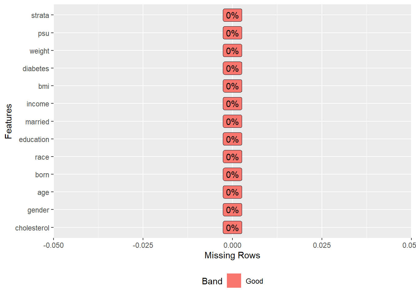
Preparing factor and continuous variables appropriately
vars = c("cholesterol", "gender", "born", "race", "education",
         "married", "income", "bmi", "diabetes")
numeric.names <- c("cholesterol", "bmi")
factor.names <- vars[!vars %in% numeric.names]

anadata[factor.names] <- apply(X = anadata[factor.names],
                               MARGIN = 2, FUN = as.factor)

anadata[numeric.names] <- apply(X = anadata[numeric.names],
                                MARGIN = 2, FUN =function (x)
                                  as.numeric(as.character(x)))
Table 1
library(tableone)
tab1 <- CreateTableOne(data = anadata, includeNA = TRUE, vars = vars)
print(tab1, showAllLevels = TRUE,  varLabels = TRUE)
#>
#>                           level              Overall
#>   n                                            1267
#>   cholesterol (mean (SD))                    193.10 (43.22)
#>   gender (%)              Female                496 (39.1)
#>                           Male                  771 (60.9)
#>   born (%)                Born.in.US            991 (78.2)
#>                           Others                276 (21.8)
#>   race (%)                Black                 246 (19.4)
#>                           Hispanic              337 (26.6)
#>                           Other                 132 (10.4)
#>                           White                 552 (43.6)
#>   education (%)           College               648 (51.1)
#>                           High.School           523 (41.3)
#>                           School                 96 ( 7.6)
#>   married (%)             Married               751 (59.3)
#>                           Never.married         226 (17.8)
#>                           Previously.married    290 (22.9)
#>   income (%)              <25k                  344 (27.2)
#>                           Between.25kto54k      435 (34.3)
#>                           Between.55kto99k      297 (23.4)
#>                           Over100k              191 (15.1)
#>   bmi (mean (SD))                             29.58 (6.84)
#>   diabetes (%)            No                   1064 (84.0)
#>                           Yes                   203 (16.0)
Linear regression when cholesterol is continuous
Fit a linear regression, and report the VIFs.
#Fitting initial regression

fit0 <- lm(cholesterol ~ gender + born + race + education +
              married + income + bmi + diabetes,
            data = anadata)

library(Publish)
publish(fit0)
#>     Variable              Units Coefficient           CI.95    p-value
#>  (Intercept)                         198.90 [184.82;212.97]    < 1e-04
#>       gender             Female         Ref
#>                            Male       -6.82  [-11.76;-1.89]   0.006854
#>         born         Born.in.US         Ref
#>                          Others       15.65    [8.54;22.75]    < 1e-04
#>         race              Black         Ref
#>                        Hispanic       -2.75   [-10.61;5.10]   0.492333
#>                           Other       -3.95   [-13.61;5.72]   0.423740
#>                           White        5.36   [-1.20;11.92]   0.109403
#>    education            College         Ref
#>                     High.School        3.51    [-1.61;8.63]   0.179871
#>                          School        0.31   [-9.63;10.24]   0.951841
#>      married            Married         Ref
#>                   Never.married      -11.05  [-17.67;-4.44]   0.001082
#>              Previously.married        4.72   [-1.43;10.86]   0.132468
#>       income               <25k         Ref
#>                Between.25kto54k       -0.48    [-6.72;5.75]   0.879480
#>                Between.55kto99k        3.41   [-3.60;10.43]   0.340491
#>                        Over100k        2.24   [-6.02;10.51]   0.595131
#>          bmi                          -0.21    [-0.56;0.15]   0.257105
#>     diabetes                 No         Ref
#>                             Yes      -10.61  [-17.21;-4.02]   0.001652

#Checking VIFs
car::vif(fit0)
#>               GVIF Df GVIF^(1/(2*Df))
#> gender    1.065810  1        1.032381
#> born      1.578258  1        1.256288
#> race      1.684064  3        1.090753
#> education 1.280113  2        1.063683
#> married   1.225520  2        1.052156
#> income    1.277005  3        1.041595
#> bmi       1.086953  1        1.042570
#> diabetes  1.073619  1        1.036156
All VIFs are small.
Test of association when cholesterol is binary
Dichotomize the outcome such that cholesterol<200 is labeled as ‘healthy’; otherwise label it as ‘unhealthy’, and name it ‘cholesterol.bin’. Test the association between this binary variable and gender.
#Creating binary variable for cholesterol
anadata$cholesterol.bin <- ifelse(anadata$cholesterol <200, "healthy", "unhealthy")
#If cholesterol is <200, then "healthy", if not, "unhealthy"

table(anadata$cholesterol.bin)
#>
#>   healthy unhealthy
#>       738       529
anadata$cholesterol.bin <- as.factor(anadata$cholesterol.bin)
anadata$cholesterol.bin <- relevel(anadata$cholesterol.bin, ref = "unhealthy")
Test of association between cholesterol and gender (no survey features)
Setting up survey design
require(survey)
summary(anadata$weight)
#>    Min. 1st Qu.  Median    Mean 3rd Qu.    Max.
#>    5470   19540   30335   48904   63822  224892
w.design <- svydesign(id = ~psu, weights = ~weight, strata = ~strata,
                      nest = TRUE, data = anadata)
summary(weights(w.design))
#>    Min. 1st Qu.  Median    Mean 3rd Qu.    Max.
#>    5470   19540   30335   48904   63822  224892
Test of association accounting for survey design
#Rao-Scott modifications (chi-sq)
svychisq(~cholesterol.bin + gender, design = w.design, statistic = "Chisq")
#>
#>  Pearson's X^2: Rao & Scott adjustment
#>
#> data:  svychisq(~cholesterol.bin + gender, design = w.design, statistic = "Chisq")
#> X-squared = 11.092, df = 1, p-value = 0.02365

#Thomas-Rao modifications (F)
svychisq(~cholesterol.bin + gender, design = w.design, statistic = "F")
#>
#>  Pearson's X^2: Rao & Scott adjustment
#>
#> data:  svychisq(~cholesterol.bin + gender, design = w.design, statistic = "F")
#> F = 5.1205, ndf = 1, ddf = 15, p-value = 0.03891
All three tests indicate strong evidence to reject the H0. There seems to be an association between gender and cholesterol level (healthy/unhealthy)
Table 1
Create a Table 1 (summarizing the covariates) stratified by the binary outcome: cholesterol.bin, utilizing the above survey features.
# Creating Table 1 stratified by binary outcome (cholesterol)
# Using the survey features

vars2 = c("gender", "born", "race", "education",
         "married", "income", "bmi", "diabetes")


kableone <- function(x, ...) {
  capture.output(x <- print(x, showAllLevels= TRUE, padColnames = TRUE, insertLevel = TRUE))
  knitr::kable(x, ...)
}
kableone(svyCreateTableOne(var = vars2, strata= "cholesterol.bin", data=w.design, test = TRUE)) | level | unhealthy | healthy | p | test | |
|---|---|---|---|---|---|
| n | 27369732.3 | 34591444.0 | |||
| gender (%) | Female | 13573865.5 (49.6) | 13917447.5 (40.2) | 0.039 | |
| Male | 13795866.8 (50.4) | 20673996.5 (59.8) | |||
| born (%) | Born.in.US | 23772751.7 (86.9) | 31532673.3 (91.2) | 0.028 | |
| Others | 3596980.6 (13.1) | 3058770.7 ( 8.8) | |||
| race (%) | Black | 1832118.3 ( 6.7) | 3696893.4 (10.7) | 0.015 | |
| Hispanic | 3263992.3 (11.9) | 3921344.6 (11.3) | |||
| Other | 1887156.6 ( 6.9) | 2601870.3 ( 7.5) | |||
| White | 20386465.2 (74.5) | 24371335.7 (70.5) | |||
| education (%) | College | 15855712.5 (57.9) | 20945710.7 (60.6) | 0.522 | |
| High.School | 10615218.7 (38.8) | 12434827.2 (35.9) | |||
| School | 898801.1 ( 3.3) | 1210906.1 ( 3.5) | |||
| married (%) | Married | 17489306.2 (63.9) | 21170020.0 (61.2) | 0.005 | |
| Never.married | 3086474.4 (11.3) | 7175237.2 (20.7) | |||
| Previously.married | 6793951.8 (24.8) | 6246186.8 (18.1) | |||
| income (%) | <25k | 4760281.8 (17.4) | 6364208.6 (18.4) | 0.915 | |
| Between.25kto54k | 8682481.6 (31.7) | 10786198.6 (31.2) | |||
| Between.55kto99k | 6939847.0 (25.4) | 9190388.2 (26.6) | |||
| Over100k | 6987121.9 (25.5) | 8250648.6 (23.9) | |||
| bmi (mean (SD)) | 29.35 (6.13) | 29.64 (7.05) | 0.593 | ||
| diabetes (%) | No | 25080412.0 (91.6) | 30006523.6 (86.7) | 0.012 | |
| Yes | 2289320.3 ( 8.4) | 4584920.4 (13.3) |
Logistic regression model
Run a logistic regression model using the same variables, utilizing the survey features. Report the corresponding odds ratios and the 95% confidence intervals.
formula1 <- as.formula(I(cholesterol.bin=="unhealthy") ~ gender + born +
                         race + education + married + income + bmi +
                         diabetes)

fit1 <- svyglm(formula1,
               design = w.design,
               family = binomial(link = "logit"))

publish(fit1)
#>   Variable              Units OddsRatio       CI.95  p-value
#>     gender             Female       Ref
#>                          Male      0.70 [0.49;0.98]   0.2866
#>       born         Born.in.US       Ref
#>                        Others      2.10 [1.41;3.13]   0.1707
#>       race              Black       Ref
#>                      Hispanic      1.15 [0.80;1.67]   0.5871
#>                         Other      1.11 [0.69;1.80]   0.7406
#>                         White      1.46 [1.00;2.14]   0.3003
#>  education            College       Ref
#>                   High.School      1.21 [0.96;1.52]   0.3563
#>                        School      0.86 [0.52;1.43]   0.6712
#>    married            Married       Ref
#>                 Never.married      0.54 [0.32;0.90]   0.2526
#>            Previously.married      1.31 [0.92;1.87]   0.3704
#>     income               <25k       Ref
#>              Between.25kto54k      1.03 [0.61;1.73]   0.9408
#>              Between.55kto99k      1.02 [0.66;1.56]   0.9525
#>                      Over100k      1.12 [0.73;1.72]   0.6920
#>        bmi                         1.00 [0.97;1.03]   0.9361
#>   diabetes                 No       Ref
#>                           Yes      0.62 [0.41;0.95]   0.2720
Wald test (survey version)
Perform a Wald test (survey version) to test the null hypothesis that all coefficients associated with the income variable are zero, and interpret.
The Wald test here gives a large p-value; We do not have evidence to reject the H0 of coefficient being 0. If the coefficient for income variable is 0, this means that the outcome in the model (cholesterol) is not affected by income. This suggests that removing income from the model does not statistically improve the model fit. So we can remove income variable from the model.
Backward elimination
Run a backward elimination (using the AIC criteria) on the above logistic regression fit (keeping important variables gender, race, bmi, diabetes in the model), and report the odds ratios and the 95% confidence intervals from the resulting final logistic regression fit.
#Running backward elimination based on AIC
require(MASS)
scope <- list(upper = ~ gender + born + race + education +
                married + income + bmi + diabetes,
              lower = ~ gender + race + bmi + diabetes)

fit3 <- step(fit1, scope = scope, trace = FALSE,
                k = 2, direction = "backward")

#Odds Ratios
publish(fit3)
#>  Variable              Units OddsRatio       CI.95   p-value
#>    gender             Female       Ref
#>                         Male      0.71 [0.51;0.98]   0.08558
#>      born         Born.in.US       Ref
#>                       Others      2.01 [1.37;2.96]   0.01184
#>      race              Black       Ref
#>                     Hispanic      1.15 [0.81;1.65]   0.46785
#>                        Other      1.11 [0.68;1.81]   0.69539
#>                        White      1.46 [0.99;2.17]   0.10469
#>   married            Married       Ref
#>                Never.married      0.54 [0.32;0.90]   0.05770
#>           Previously.married      1.30 [0.93;1.80]   0.17125
#>       bmi                         1.00 [0.97;1.03]   0.95146
#>  diabetes                 No       Ref
#>                          Yes      0.61 [0.40;0.91]   0.05445
Born and married are also found to be useful on top of gender + race + bmi + diabetes.
Interaction terms
Checking interaction terms
– gender and whether married
– gender and whether born in the US
– gender and diabetes
– whether married and diabetes
#gender and married
fit4 <- update(fit3, .~. + interaction(gender, married))
anova(fit3, fit4)
#> Working (Rao-Scott+F) LRT for interaction(gender, married)
#>  in svyglm(formula = I(cholesterol.bin == "unhealthy") ~ gender +
#>     born + race + married + bmi + diabetes + interaction(gender,
#>     married), design = w.design, family = binomial(link = "logit"))
#> Working 2logLR =  0.7461308 p= 0.70903
#> (scale factors:  1.1 0.93 );  denominator df= 4
Do not include interaction term
#gender and born in us
fit5 <- update(fit3, .~. + interaction(gender, born))
anova(fit3, fit5)
#> Working (Rao-Scott+F) LRT for interaction(gender, born)
#>  in svyglm(formula = I(cholesterol.bin == "unhealthy") ~ gender +
#>     born + race + married + bmi + diabetes + interaction(gender,
#>     born), design = w.design, family = binomial(link = "logit"))
#> Working 2logLR =  0.4635299 p= 0.52441
#> df=1;  denominator df= 5
Do not include interaction term
#gender and diabetes
fit6 <- update(fit3, .~. + interaction(gender, diabetes))
anova(fit3, fit6)
#> Working (Rao-Scott+F) LRT for interaction(gender, diabetes)
#>  in svyglm(formula = I(cholesterol.bin == "unhealthy") ~ gender +
#>     born + race + married + bmi + diabetes + interaction(gender,
#>     diabetes), design = w.design, family = binomial(link = "logit"))
#> Working 2logLR =  1.222596 p= 0.32211
#> df=1;  denominator df= 5
Do not include interaction term
#married and diabetes
fit7 <- update(fit3, .~. + interaction(married, diabetes))
anova(fit3, fit7)
#> Working (Rao-Scott+F) LRT for interaction(married, diabetes)
#>  in svyglm(formula = I(cholesterol.bin == "unhealthy") ~ gender +
#>     born + race + married + bmi + diabetes + interaction(married,
#>     diabetes), design = w.design, family = binomial(link = "logit"))
#> Working 2logLR =  0.3207507 p= 0.84547
#> (scale factors:  1.4 0.62 );  denominator df= 4
Do not include interaction term
None of the interaction terms are improving the model fit.
AUC
Report AUC of the final model (only using weight argument) and interpret.
AUC of the final model (only using weight argument) and interpret
require(ROCR)
# WeightedROC may not be on cran for all R versions
# devtools::install_github("tdhock/WeightedROC")

library(WeightedROC)
svyROCw <- function(fit = fit3, outcome = anadata$cholesterol.bin == "unhealthy", weight = anadata$weight){
  if (is.null(weight)){ # require(ROCR)
    prob <- predict(fit, type = "response")
  pred <- prediction(as.vector(prob), outcome)
  perf <- performance(pred, "tpr", "fpr")
  auc <- performance(pred, measure = "auc")
  auc <- auc@y.values[[1]]
  roc.data <- data.frame(fpr = unlist(perf@x.values), tpr = unlist(perf@y.values),
      model = "Logistic")
  with(data = roc.data,plot(fpr, tpr, type="l", xlim=c(0,1), ylim=c(0,1), lwd=1,
     xlab="1 - specificity", ylab="Sensitivity",
     main = paste("AUC = ", round(auc,3))))
  mtext("Unweighted ROC")
  abline(0,1, lty=2)
  } else {
    outcome <- as.numeric(outcome)
  pred <- predict(fit, type = "response")
  tp.fp <- WeightedROC(pred, outcome, weight)
  auc <- WeightedAUC(tp.fp)
  with(data = tp.fp,plot(FPR, TPR, type="l", xlim=c(0,1), ylim=c(0,1), lwd=1,
     xlab="1 - specificity", ylab="Sensitivity",
     main = paste("AUC = ", round(auc,3))))
  abline(0,1, lty=2)
  mtext("Weighted ROC")
  }
}
svyROCw(fit = fit3, outcome = anadata$cholesterol.bin == "unhealthy", weight = anadata$weight)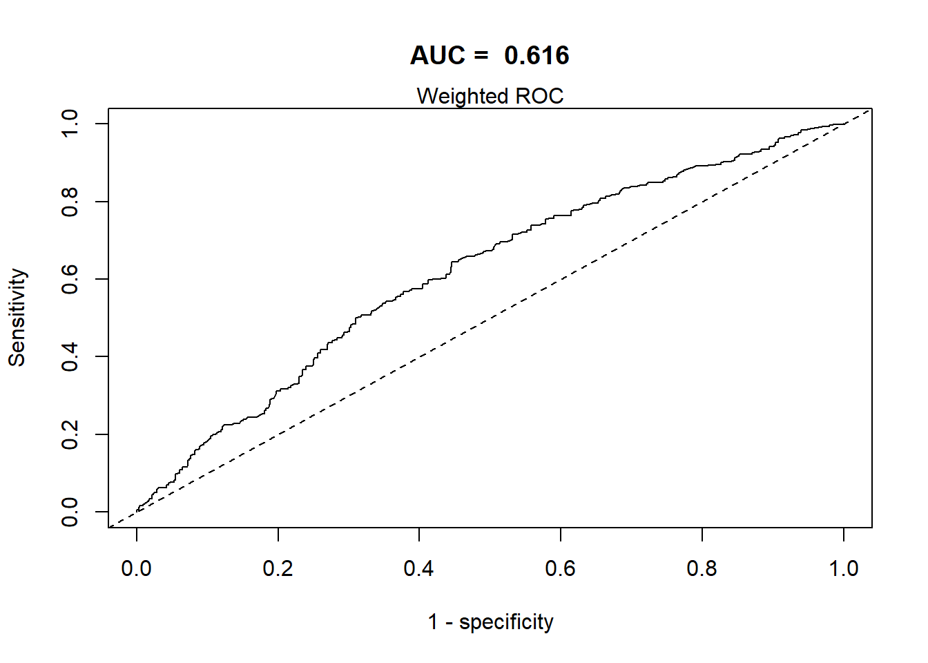
The area under the curve in the final model is 0.611, using the survey weighted ROC. The AUC of 0.611 indicates that this model has poor discrimination.
Archer-Lemeshow Goodness of fit
Report Archer-Lemeshow Goodness of fit test and interpret (utilizing all the survey features).
#Archer-Lemeshow Goodness of fit test utilizing all survey features
AL.gof2 <- function(fit = fit3, data = anadata,
                   weight = "weight", psu = "psu", strata = "strata"){
  r <- residuals(fit, type = "response")
  f<-fitted(fit)
  breaks.g <- c(-Inf, quantile(f, (1:9)/10), Inf)
  breaks.g <- breaks.g + seq_along(breaks.g) * .Machine$double.eps
  g<- cut(f, breaks.g)
  data2g <- cbind(data,r,g)
  newdesign <- svydesign(id=as.formula(paste0("~",psu)),
                         strata=as.formula(paste0("~",strata)),
                         weights=as.formula(paste0("~",weight)),
                         data=data2g, nest = TRUE)
  decilemodel <- svyglm(r~g, design=newdesign)
  res <- regTermTest(decilemodel, ~g)
  return(res)
}

AL.gof2(fit3, anadata, weight = "weight", psu = "psu", strata = "strata")
#> Wald test for g
#>  in svyglm(formula = r ~ g, design = newdesign)
#> F =  0.7569326  on  9  and  6  df: p= 0.66075
Archer and Lemeshow GoF test was used to test the fit of this model. The p-value of 0.3043, which is greater than 0.05. This means that there is no evidence of lack of fit to this model.
Add age as a predictor for linear regression
Fit another logistic regression (similar to Q1) with the above-mentioned predictors (as obtained in Q7) and age, utilizing the survey features. What difference do you see from the previous fit results?
aic.int.model <- eval(fit3$call[[2]])
aic.int.model
#> I(cholesterol.bin == "unhealthy") ~ gender + born + race + married +
#>     bmi + diabetes

formula3 <- as.formula(cholesterol.bin ~ gender + born + race + married + bmi + diabetes + age)
fit9 <- svyglm(formula3,
               design = w.design,
               family = binomial(link="logit"))
summary(fit9)
#>
#> Call:
#> svyglm(formula = formula3, design = w.design, family = binomial(link = "logit"))
#>
#> Survey design:
#> svydesign(id = ~psu, weights = ~weight, strata = ~strata, nest = TRUE,
#>     data = anadata)
#>
#> Coefficients:
#>                             Estimate Std. Error t value Pr(>|t|)
#> (Intercept)                1.0657919  0.6260889   1.702   0.1494
#> genderMale                 0.3821902  0.1703394   2.244   0.0749 .
#> bornOthers                -0.6912102  0.2026407  -3.411   0.0190 *
#> raceHispanic              -0.2442019  0.1823190  -1.339   0.2381
#> raceOther                 -0.1570271  0.2306208  -0.681   0.5262
#> raceWhite                 -0.3638735  0.2029676  -1.793   0.1330
#> marriedNever.married       0.4029107  0.2637962   1.527   0.1872
#> marriedPreviously.married -0.2096009  0.1620478  -1.293   0.2524
#> bmi                       -0.0002237  0.0134117  -0.017   0.9873
#> diabetesYes                0.6534019  0.2456333   2.660   0.0449 *
#> age                       -0.0151364  0.0042038  -3.601   0.0155 *
#> ---
#> Signif. codes:  0 '***' 0.001 '**' 0.01 '*' 0.05 '.' 0.1 ' ' 1
#>
#> (Dispersion parameter for binomial family taken to be 1.000456)
#>
#> Number of Fisher Scoring iterations: 4
publish(fit9)
#>  Variable              Units OddsRatio       CI.95   p-value
#>    gender             Female       Ref
#>                         Male      1.47 [1.05;2.05]   0.07487
#>      born         Born.in.US       Ref
#>                       Others      0.50 [0.34;0.75]   0.01902
#>      race              Black       Ref
#>                     Hispanic      0.78 [0.55;1.12]   0.23809
#>                        Other      0.85 [0.54;1.34]   0.52619
#>                        White      0.69 [0.47;1.03]   0.13299
#>   married            Married       Ref
#>                Never.married      1.50 [0.89;2.51]   0.18721
#>           Previously.married      0.81 [0.59;1.11]   0.25238
#>       bmi                         1.00 [0.97;1.03]   0.98734
#>  diabetes                 No       Ref
#>                          Yes      1.92 [1.19;3.11]   0.04488
#>       age                         0.98 [0.98;0.99]   0.01553
Comparing with previous model fit
publish(fit3)
#>  Variable              Units OddsRatio       CI.95   p-value
#>    gender             Female       Ref
#>                         Male      0.71 [0.51;0.98]   0.08558
#>      born         Born.in.US       Ref
#>                       Others      2.01 [1.37;2.96]   0.01184
#>      race              Black       Ref
#>                     Hispanic      1.15 [0.81;1.65]   0.46785
#>                        Other      1.11 [0.68;1.81]   0.69539
#>                        White      1.46 [0.99;2.17]   0.10469
#>   married            Married       Ref
#>                Never.married      0.54 [0.32;0.90]   0.05770
#>           Previously.married      1.30 [0.93;1.80]   0.17125
#>       bmi                         1.00 [0.97;1.03]   0.95146
#>  diabetes                 No       Ref
#>                          Yes      0.61 [0.40;0.91]   0.05445
publish(fit9)
#>  Variable              Units OddsRatio       CI.95   p-value
#>    gender             Female       Ref
#>                         Male      1.47 [1.05;2.05]   0.07487
#>      born         Born.in.US       Ref
#>                       Others      0.50 [0.34;0.75]   0.01902
#>      race              Black       Ref
#>                     Hispanic      0.78 [0.55;1.12]   0.23809
#>                        Other      0.85 [0.54;1.34]   0.52619
#>                        White      0.69 [0.47;1.03]   0.13299
#>   married            Married       Ref
#>                Never.married      1.50 [0.89;2.51]   0.18721
#>           Previously.married      0.81 [0.59;1.11]   0.25238
#>       bmi                         1.00 [0.97;1.03]   0.98734
#>  diabetes                 No       Ref
#>                          Yes      1.92 [1.19;3.11]   0.04488
#>       age                         0.98 [0.98;0.99]   0.01553
AIC(fit3)
#>       eff.p         AIC    deltabar
#>   11.121795 1706.792543    1.235755
AIC(fit9)
#>      eff.p        AIC   deltabar
#>   12.14310 1694.15974    1.21431
Both models are fitted with the binomial family and fit3 is nested within fit9 (the latter simply adds age), so their AIC values are directly comparable. The model with age (fit9) returns the lower AIC, indicating that adding age improves the design-based fit. Note that AIC.svyglm reports the design-based AIC of Lumley and Scott (2015) (the Lumley-Scott AIC), which adjusts the usual penalty for the complex survey design rather than using the naive number of parameters.
Video content (optional)
For those who prefer a video walkthrough, feel free to watch the video below, which offers a description of an earlier version of the above content.