Change-in-estimate

The change-in-estimate criterion is one of the purposeful variable selection criteria, where a relative change is used to determine whether a variable should be included in the model or omitted from the model. This change can be measured by using the relative change in the regression coefficient or relative change by adjusting the effect of the variance estimate. Eliminating a variable using this technique can bias the estimates. In particular, this method is not appropriate when the estimate is non-collapsible. In this chapter, we will see the use of change-in-estimate for various measures of effects (RD and OR, and impact of collapsibility vs non-collapsibility in absence of confounding).

For a collapsible measure (e.g., beta coefficient from a linear model with a continuous outcome, risk difference or risk ratio from a generalized linear model with a binary outcome), our estimate could be the same when we adjust our model or not for a variable that is not a confounder. However, a non-collapsible measure (e.g., odds ratio) could be different whether or not we adjust our model for a variable that is not a confounder.

# Load required packages
library(simcausal)

Adjusting for a variable that is a confounder

Continuous Outcome

True treatment effect = 1.3

Data generating process

require(simcausal)
D <- DAG.empty()
D <- D + 
  node("L", distr = "rnorm", mean = 0, sd = 1) + 
  node("A", distr = "rnorm", mean = 0 + L, sd = 1) + 
  node("P", distr = "rbern", prob = plogis(-10)) + 
  node("Y", distr = "rnorm", mean = 1.1 * L + 1.3 * A, sd = .1)
Dset <- set.DAG(D)

Generate DAG

plotDAG(Dset, xjitter = 0.1, yjitter = .9,
        edge_attrs = list(width = 0.5, arrow.width = 0.4, arrow.size = 0.7),
        vertex_attrs = list(size = 12, label.cex = 0.8))

Generate Data

require(simcausal)
Obs.Data <- sim(DAG = Dset, n = 1000000, rndseed = 123)
head(Obs.Data)

Estimate effect (beta-coef)

fit <- glm(Y ~ A, family="gaussian", data=Obs.Data)
round(coef(fit),2)
#> (Intercept)           A 
#>        0.00        1.85

fit2 <- glm(Y ~ A + L, family="gaussian", data=Obs.Data)
round(coef(fit2),2)
#> (Intercept)           A           L 
#>         0.0         1.3         1.1

Including a variable that is a confounder (L) in the model changes effect estimate (1.3).

Binary Outcome

True treatment effect = 1.3

Data generating process

require(simcausal)
D <- DAG.empty()
D <- D + 
  node("L", distr = "rnorm", mean = 0, sd = 1) + 
  node("A", distr = "rnorm", mean = 0 + L, sd = 1) + 
  node("P", distr = "rbern", prob = plogis(-10)) + 
  # node("M", distr = "rnorm", mean = P + 0.5 * A, sd = 1) + 
  node("Y", distr = "rbern", prob = plogis( 1.1 * L + 1.3 * A)) 
Dset <- set.DAG(D)
#> ...automatically assigning order attribute to some nodes...
#> node L, order:1
#> node A, order:2
#> node P, order:3
#> node Y, order:4

Generate DAG

plotDAG(Dset, xjitter = 0.1, yjitter = .9,
        edge_attrs = list(width = 0.5, arrow.width = 0.4, arrow.size = 0.7),
        vertex_attrs = list(size = 12, label.cex = 0.8))
#> using the following vertex attributes:
#> 120.8NAdarkbluenone0
#> using the following edge attributes:
#> 0.50.40.7black1

Generate Data

require(simcausal)
Obs.Data <- sim(DAG = Dset, n = 1000000, rndseed = 123)
head(Obs.Data)

Estimate effect (OR)

fit <- glm(Y ~ A, family=binomial(link = "logit"), data=Obs.Data)
round(coef(fit),2)
#> (Intercept)           A 
#>        0.00        1.68

fit2 <- glm(Y ~ A + L, family=binomial(link = "logit"), data=Obs.Data)
round(coef(fit2),2)
#> (Intercept)           A           L 
#>         0.0         1.3         1.1

Including a variable that is a confounder (L) in the model changes effect estimate (1.3).

Adjusting for a variable that is not a confounder (simplified)

Continuous Outcome

True treatment effect = 1.3

Data generating process

require(simcausal)
D <- DAG.empty()
D <- D + 
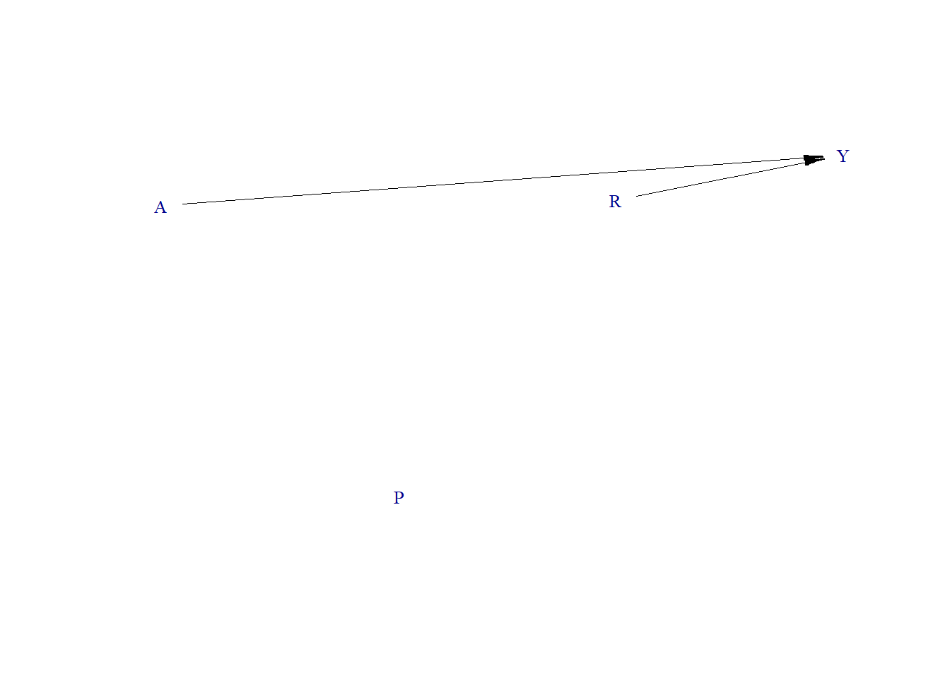
    node("A", distr = "rnorm", mean = 0, sd = 1) + 
  node("P", distr = "rbern", prob = plogis(-10)) + 
  # node("M", distr = "rnorm", mean = P + 0.5 * A, sd = 1) + 
  node("R", distr = "rnorm", mean = 0, sd = 1) + 
  node("Y", distr = "rnorm", mean = 1.1 * R + 1.3 * A, sd = .1)
Dset <- set.DAG(D)
#> ...automatically assigning order attribute to some nodes...
#> node A, order:1
#> node P, order:2
#> node R, order:3
#> node Y, order:4

Generate DAG

plotDAG(Dset, xjitter = 0.1, yjitter = .9,
        edge_attrs = list(width = 0.5, arrow.width = 0.4, arrow.size = 0.7),
        vertex_attrs = list(size = 12, label.cex = 0.8))
#> using the following vertex attributes:
#> 120.8NAdarkbluenone0
#> using the following edge attributes:
#> 0.50.40.7black1

Generate Data

require(simcausal)
Obs.Data <- sim(DAG = Dset, n = 1000000, rndseed = 123)
head(Obs.Data)

Estimate effect (beta-coef)

fit <- glm(Y ~ A, family="gaussian", data=Obs.Data)
round(coef(fit),2)
#> (Intercept)           A 
#>         0.0         1.3

fit2 <- glm(Y ~ A + R, family="gaussian", data=Obs.Data)
round(coef(fit2),2)
#> (Intercept)           A           R 
#>         0.0         1.3         1.1

Including a variable that is not a confounder (R is a pure risk factor for the outcome Y) in the model does not change effect estimate (1.3).

Binary Outcome

True treatment effect = 1.3

Data generating process

require(simcausal)
D <- DAG.empty()
D <- D + 
  node("A", distr = "rnorm", mean = 0, sd = 1) + 
  node("P", distr = "rbern", prob = plogis(-10)) + 
  # node("M", distr = "rnorm", mean = P + 0.5 * A, sd = 1) + 
  node("R", distr = "rnorm", mean = 0, sd = 1) + 
  node("Y", distr = "rbern", prob = plogis(1.1 * R + 1.3 * A)) 
Dset <- set.DAG(D)
#> ...automatically assigning order attribute to some nodes...
#> node A, order:1
#> node P, order:2
#> node R, order:3
#> node Y, order:4

Generate DAG

plotDAG(Dset, xjitter = 0.1, yjitter = .9,
        edge_attrs = list(width = 0.5, arrow.width = 0.4, arrow.size = 0.7),
        vertex_attrs = list(size = 12, label.cex = 0.8))
#> using the following vertex attributes:
#> 120.8NAdarkbluenone0
#> using the following edge attributes:
#> 0.50.40.7black1

Generate Data

require(simcausal)
Obs.Data <- sim(DAG = Dset, n = 1000000, rndseed = 123)
head(Obs.Data)

Estimate effect (OR)

fit <- glm(Y ~ A, family=binomial(link = "logit"), data=Obs.Data)
round(coef(fit),2)
#> (Intercept)           A 
#>        0.00        1.06

fit2 <- glm(Y ~ A + R, family=binomial(link = "logit"), data=Obs.Data)
round(coef(fit2),2)
#> (Intercept)           A           R 
#>         0.0         1.3         1.1

Including a variable that is not a confounder (R is a pure risk factor for the outcome Y) in the model changes effect estimate (1.3).

Adjusting for a variable that is not a confounder (Complex)

Continuous Outcome

True treatment effect = 1.3

Data generating process

require(simcausal)
D <- DAG.empty()
D <- D + 
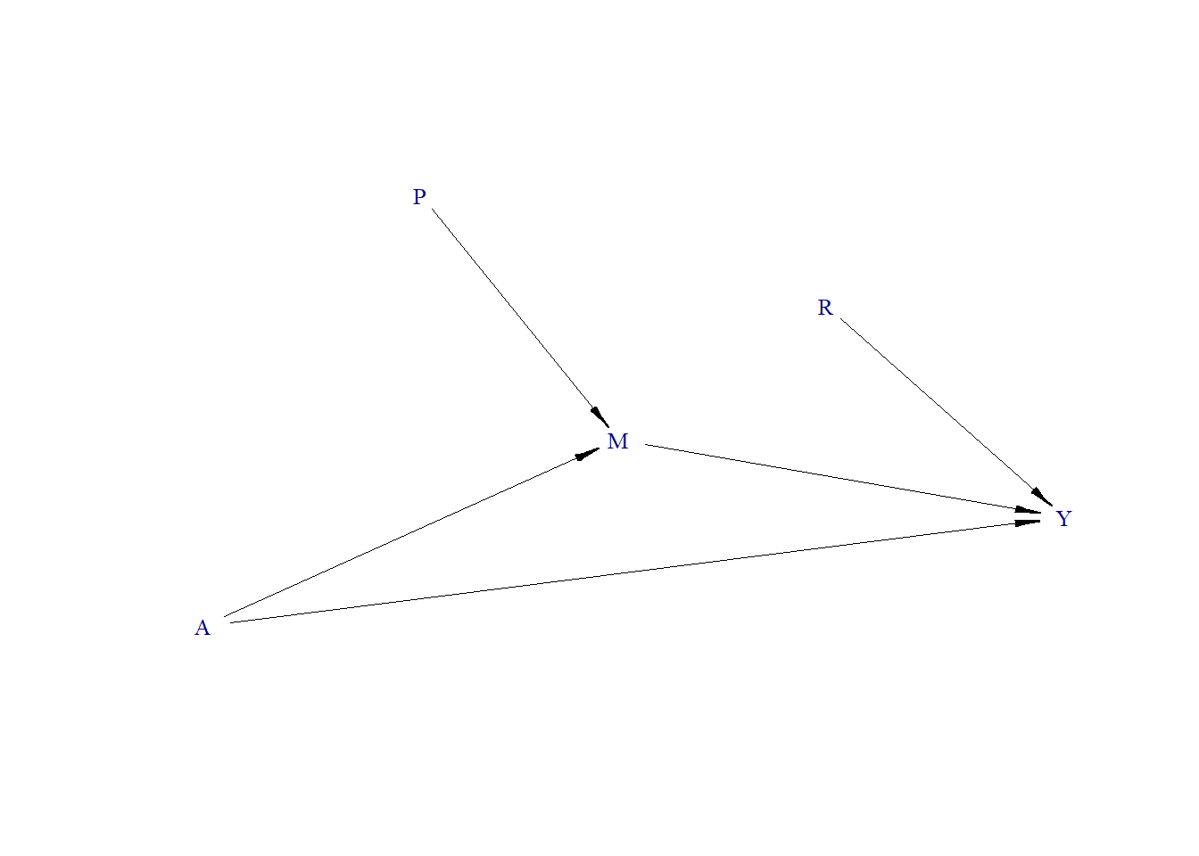
    node("A", distr = "rnorm", mean = 0, sd = 1) + 
  node("P", distr = "rbern", prob = plogis(-10)) + 
  node("M", distr = "rnorm", mean = P + 0.5 * A, sd = 1) + 
  node("R", distr = "rnorm", mean = 0, sd = 1) + 
  node("Y", distr = "rnorm", mean = 0.5 * M + 1.1 * R + 1.3 * A, sd = .1)
Dset <- set.DAG(D)
#> ...automatically assigning order attribute to some nodes...
#> node A, order:1
#> node P, order:2
#> node M, order:3
#> node R, order:4
#> node Y, order:5

Generate DAG

plotDAG(Dset, xjitter = 0.1, yjitter = .9,
        edge_attrs = list(width = 0.5, arrow.width = 0.4, arrow.size = 0.7),
        vertex_attrs = list(size = 12, label.cex = 0.8))
#> using the following vertex attributes:
#> 120.8NAdarkbluenone0
#> using the following edge attributes:
#> 0.50.40.7black1

Generate Data

require(simcausal)
Obs.Data <- sim(DAG = Dset, n = 1000000, rndseed = 123)
head(Obs.Data)

Estimate effect (beta-coef)

fit <- glm(Y ~ A + M, family="gaussian", data=Obs.Data)
round(coef(fit),2)
#> (Intercept)           A           M 
#>         0.0         1.3         0.5

fit2 <- glm(Y ~ A + M + R, family="gaussian", data=Obs.Data)
round(coef(fit2),2)
#> (Intercept)           A           M           R 
#>         0.0         1.3         0.5         1.1

Including a variable that is not a confounder (R is a pure risk factor for the outcome Y) in the model does not change effect estimate (1.3).

Binary Outcome

True treatment effect = 1.3

Data generating process

require(simcausal)
D <- DAG.empty()
D <- D + 
  node("A", distr = "rnorm", mean = 0, sd = 1) + 
  node("P", distr = "rbern", prob = plogis(-10)) + 
  node("M", distr = "rnorm", mean = P + 0.5 * A, sd = 1) + 
  node("R", distr = "rnorm", mean = 0, sd = 1) + 
  node("Y", distr = "rbern", prob = plogis(0.5 * M + 1.1 * R + 1.3 * A)) 
Dset <- set.DAG(D)
#> ...automatically assigning order attribute to some nodes...
#> node A, order:1
#> node P, order:2
#> node M, order:3
#> node R, order:4
#> node Y, order:5

Generate DAG

plotDAG(Dset, xjitter = 0.1, yjitter = .9,
        edge_attrs = list(width = 0.5, arrow.width = 0.4, arrow.size = 0.7),
        vertex_attrs = list(size = 12, label.cex = 0.8))
#> using the following vertex attributes:
#> 120.8NAdarkbluenone0
#> using the following edge attributes:
#> 0.50.40.7black1

Generate Data

require(simcausal)
Obs.Data <- sim(DAG = Dset, n = 1000000, rndseed = 123)
head(Obs.Data)

Estimate effect (OR)

fit <- glm(Y ~ A + M, family=binomial(link = "logit"), data=Obs.Data)
round(coef(fit),2)
#> (Intercept)           A           M 
#>        0.00        1.06        0.41

fit2 <- glm(Y ~ A + M + R, family=binomial(link = "logit"), data=Obs.Data)
round(coef(fit2),2)
#> (Intercept)           A           M           R 
#>        0.00        1.29        0.50        1.10

Including a variable that is not a confounder (R is a pure risk factor for the outcome Y) in the model changes effect estimate (1.3).

Video content (optional)

Tip

For those who prefer a video walkthrough, feel free to watch the video below, which offers a description of an earlier version of the above content.