Confounding

This tutorial aims to delve into the role of confounding variables in data analysis, especially in the context of big data. We will examine each of these using simulations built on Directed Acyclic Graphs (DAGs). The objective is to understand whether a simple regression adjusting for the confounder variable can correctly estimate treatment effects in such a large sample.

# devtools::install_github('osofr/simcausal')
require(simcausal)

Big data: What if we had 1,000,000 (one million) observations? Would that give us true result? Let’s try to answer that using DAGs.

Let us consider

L is continuous variable
A is binary treatment
Y is continuous outcome

An example of A could be receiving the right heart catheterization (RHC) procedure or not, Y could be the length of hospital stay, and L could be age (see here).

Non-null effect

True treatment effect = 1.3

Data generating process

To perform the lab, we’ll need the simcausal R package. This package may not be available on CRAN but can be installed from the author’s GitHub page.

require(simcausal)
D <- DAG.empty()
D <- D + 
  node("L", distr = "rnorm", mean = 10, sd = 1) + 
  node("A", distr = "rbern", prob = plogis(-10 + 1.1*L)) +
  node("Y", distr = "rnorm", mean = 0.5 * L + 1.3 * A, sd = 0.1)
Dset <- set.DAG(D)

Note that rnorm and rbern generate random samples from Normal and Bernoulli distributions, respectively. In the above code chuck, we set the parameters to generate L from Normal distribution with a mean of 10 and a standard deviation of 1. Similarly, we set the parameters to generate A from the Bernoulli distribution with the probability of logit of (-10 + 1.1 \(\times\) L). Finally, we set the parameters to generate Y from the Normal distribution with a mean of (0.5 \(\times\) L + 1.3 \(\times\) A) and a standard deviation of 0.1.

Generate DAG

Let us draw a directed acyclic graph (DAG). Below we use the plotDAG function from the simcausal package. However, we can draw a DAG using DAGitty.

plotDAG(Dset, xjitter = 0.1, yjitter = .9,
        edge_attrs = list(width = 0.5, arrow.width = 0.4, arrow.size = 0.7),
        vertex_attrs = list(size = 12, label.cex = 0.8))
#> using the following vertex attributes:
#> 120.8NAdarkbluenone0
#> using the following edge attributes:
#> 0.50.40.7black1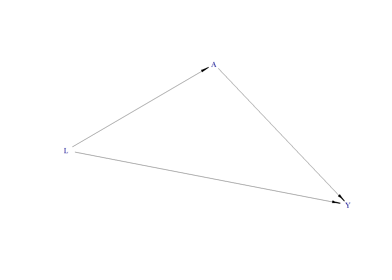

As per the DAG, L is a confounder. When exploring the relationship between A and Y, we need to adjust our model for L to get an unbiased estimate of A on Y.

Generate Data

Now, let us simulate the data using the defined parameters and the DAG. Below, we generate data for 1,000,000 participants. We set a seed 123 so that one can reproduce the same dataset.

require(simcausal)
Obs.Data <- sim(DAG = Dset, n = 1000000, rndseed = 123)
head(Obs.Data)

Estimate effect

Now we will fit the generalized linear model (glm), without and with adjusting for L.

# Not adjusted for L
fit0 <- glm(Y ~ A, family="gaussian", data=Obs.Data)
round(coef(fit0),2)
#> (Intercept)           A 
#>        4.69        1.75

# Adjusted for L
fit <- glm(Y ~ A + L, family="gaussian", data=Obs.Data)
round(coef(fit),2)
#> (Intercept)           A           L 
#>         0.0         1.3         0.5

Important

In this case, our true treatment effect is 1.3. When we estimate the relationship between A and Y without adjusting for L, we obtain an estimated effect of 1.75. However, this is not the true effect. The true treatment effect of 1.3 is recovered when we adjust for L.

Null effect

True treatment effect = 0

Let us see the results when there is no treatment effect, i.s., the true treatment effect is zero.

Data generating process

require(simcausal)
D <- DAG.empty()
D <- D + 
  node("L", distr = "rnorm", mean = 10, sd = 1) + 
  node("A", distr = "rbern", prob = plogis(-10 + 1.1*L)) +
  node("Y", distr = "rnorm", mean = 0.5 * L + 0 * A, sd = .1)
Dset <- set.DAG(D)

Generate DAG

plotDAG(Dset, xjitter = 0.1, yjitter = .9,
        edge_attrs = list(width = 0.5, arrow.width = 0.4, arrow.size = 0.7),
        vertex_attrs = list(size = 12, label.cex = 0.8))

Generate Data

require(simcausal)
Obs.Data <- sim(DAG = Dset, n = 1000000, rndseed = 123)
head(Obs.Data)

Estimate effect

# Not adjusted for L
fit0 <- glm(Y ~ A, family = "gaussian", data = Obs.Data)
round(coef(fit0),2)
#> (Intercept)           A 
#>        4.69        0.45

# Adjusted for L
fit <- glm(Y ~ A + L, family = "gaussian", data = Obs.Data)
round(coef(fit),2)
#> (Intercept)           A           L 
#>         0.0         0.0         0.5

Important

In this second scenario, the true treatment effect is zero. There is no arrow from A to Y in the DAG, but L remains a common cause for both. Upon analyzing the data without adjusting for L, we observe an induced correlation between A and Y. This correlation disappears, confirming the true null effect, when we adjust for L.

Video content (optional)

Tip

For those who prefer a video walkthrough, feel free to watch the video below, which offers a description of an earlier version of the above content.