Baron and Kenny
Baron and Kenny (1986) approach 1
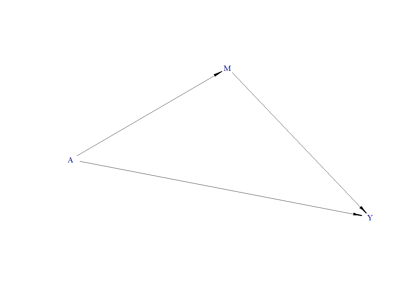
In Baron and Kenny approach 1 (Baron and Kenny 1986), two regression models are fitted to estimate the total effect, direct effect, and indirect effect.
\[ Y = \alpha_{0} + \beta_0 A + \gamma_0 M, \] \[ Y = \alpha_{1} + \beta_1 A, \] where \(Y\) is the outcome, \(A\) is the exposure, \(M\) is the mediator, and \(\alpha, \beta, \gamma\) are regression coefficients. The effects are then calculated as:
- Total effect of A on Y: \(\hat{\beta}_1\)
- Direct effect of A on Y: \(\hat{\beta}_0\)
- Indirect effect of A on Y through M: \(\hat{\beta}_1 - \hat{\beta}_0\),
where \(\hat{\beta}\) is estimated regression coefficient of \(\beta\).
Baron and Kenny (1986) approach 2
In the second approach, three models are fitted:
\[ Y = \alpha_{0} + \beta_0 A + \gamma_0 M, \] \[ Y = \alpha_{1} + \beta_1 A, \] \[ M = \alpha_{2} + \beta_2 A, \]
The indirect effect of A on Y through M can be calculated as: \(\hat{\beta}_2 \times \hat{\beta}_0\), where \(\hat{\beta}\) is estimated regression coefficient of \(\beta\).
Big data: What if we had 1,000,000 (1 million) observations?
Let us explore the mediation analysis using Baron and Kenny (1986) approaches. We first simulate a big dataset and then show the results from the mediation analysis.
Continuous outcome, continuous mediator
- True direct effect (A → Y, holding M) = 1.3
- True indirect effect (A → M → Y) = 0.5 × 0.5 = 0.25
- True total effect = direct + indirect = 1.3 + 0.25 = 1.55
Data generating process
require(simcausal)
D <- DAG.empty()
D <- D +
    node("A", distr = "rnorm", mean = 0, sd = 1) +
    node("M", distr = "rnorm", mean = 0.5 * A, sd = 1) +
    node("Y", distr = "rnorm", mean = 0.5 * M + 1.3 * A, sd = .1)
Dset <- set.DAG(D)
#> ...automatically assigning order attribute to some nodes...
#> node A, order:1
#> node M, order:2
#> node Y, order:3
Generate DAG

Generate Data
Estimate effect (beta-coef)
fit <- glm(Y ~ A, family="gaussian", data=Obs.Data)
round(coef(fit),2)
#> (Intercept)           A
#>        0.00        1.55
fit.am <- glm(Y ~ A + M, family="gaussian", data=Obs.Data)
round(coef(fit.am),2)
#> (Intercept)           A           M
#>         0.0         1.3         0.5
fit.m <- glm(M ~ A, family="gaussian", data=Obs.Data)
round(coef(fit.m),2)
#> (Intercept)           A
#> 0.0 0.5Baron and Kenny (1986) approach 1
Baron and Kenny (1986) approach 2
Binary outcome, continuous mediator
- True direct effect (A → Y, conditional on M) = 1.3 on the log-odds scale
- Because the outcome is binary, this conditional log-odds coefficient is non-collapsible: it does not transfer directly to the marginal odds ratio, and the total/indirect decomposition does not simply add up as in the linear case.
Data generating process
require(simcausal)
D <- DAG.empty()
D <- D +
  node("A", distr = "rnorm", mean = 0, sd = 1) +
  node("M", distr = "rnorm", mean = 0.5 * A, sd = 1) +
  node("Y", distr = "rbern", prob = plogis(0.5 * M + 1.3 * A))
Dset <- set.DAG(D)
#> ...automatically assigning order attribute to some nodes...
#> node A, order:1
#> node M, order:2
#> node Y, order:3
Generate DAG
Generate Data
Estimate effect (beta-coef)
fit <- glm(Y ~ A, family=binomial(link = "logit"), data=Obs.Data)
round(coef(fit),2)
#> (Intercept)           A
#>        0.00        1.48
fit.am <- glm(Y ~ A + M, family=binomial(link = "logit"), data=Obs.Data)
round(coef(fit.am),2)
#> (Intercept)           A           M
#>         0.0         1.3         0.5
fit.m <- glm(M ~ A, family="gaussian", data=Obs.Data)
round(coef(fit.m),2)
#> (Intercept)           A
#> 0.0 0.5Baron and Kenny (1986) approach 1
Baron and Kenny (1986) approach 2
Binary outcome, binary mediator
- True direct effect (A → Y, conditional on M) = 1.3 on the log-odds scale
- Again the binary outcome makes this conditional log-odds coefficient non-collapsible, so it does not transfer directly to the marginal odds ratio, and the total/indirect effects do not decompose additively.
Data generating process
require(simcausal)
D <- DAG.empty()
D <- D +
  node("A", distr = "rnorm", mean = 0, sd = 1) +
  node("M", distr = "rbern", prob = plogis(0.5 * A)) +
  node("Y", distr = "rbern", prob = plogis(0.5 * M + 1.3 * A))
Dset <- set.DAG(D)
#> ...automatically assigning order attribute to some nodes...
#> node A, order:1
#> node M, order:2
#> node Y, order:3
Generate DAG

Generate Data
Estimate effect (beta-coef)
fit <- glm(Y ~ A, family=binomial(link = "logit"), data=Obs.Data)
round(coef(fit),2)
#> (Intercept)           A
#>        0.25        1.34
fit.am <- glm(Y ~ A + M, family=binomial(link = "logit"), data=Obs.Data)
round(coef(fit.am),2)
#> (Intercept)           A           M
#>         0.0         1.3         0.5
fit.m <- glm(M ~ A, family=binomial(link = "logit"), data=Obs.Data)
round(coef(fit.m),2)
#> (Intercept)           A
#> 0.0 0.5Baron and Kenny (1986) approach 1
Baron and Kenny (1986) approach 2
As we can see, the estimated indirect effects are different from the two approaches. That means Baron and Kenny’s (1986) approach doesn’t work for a non-collapsible effect measure such as the odds ratio.
Video content (optional)
For those who prefer a video walkthrough, feel free to watch the video below, which offers a description of an earlier version of the above content.