Mediator

Mediators play a crucial role in understanding how a treatment variable affects an outcome. A mediator variable lies in the pathway between the treatment and outcome, essentially transmitting or explaining the effect of the treatment variable. In this expanded tutorial, we’ll delve into more details based on the lecture, specifically focusing on the true direct and indirect effects when a mediator is present.

# Load required packages
library(simcausal)

Let us consider

M is continuous variable
A is binary treatment
Y is continuous outcome

An example of A could be receiving the right heart catheterization (RHC) procedure or not, Y could be the length of hospital stay, and M could be the number of comorbidities.

Non-null effect

True treatment effect = 1.3

Our true treatment effect is 1.3, and the mediator variable’s effect on the outcome Y is 0.5. It’s important to differentiate between these effects.

Data generating process

require(simcausal)
D <- DAG.empty()
D <- D + 
  node("A", distr = "rbern", prob = plogis(-10)) +
  node("M", distr = "rnorm", mean = 10 + 0.9 * A, sd = 1) + 
  node("Y", distr = "rnorm", mean = 0.5 * M + 1.3 * A, sd = .1)
Dset <- set.DAG(D)

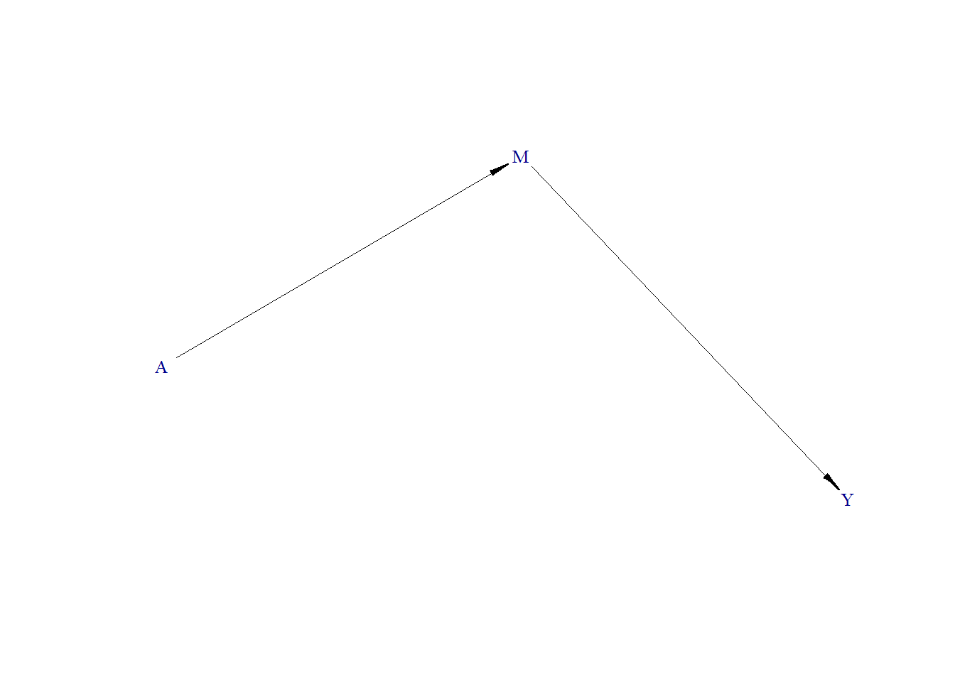
Generate DAG

plotDAG(Dset, xjitter = 0.1, yjitter = .9,
        edge_attrs = list(width = 0.5, arrow.width = 0.4, arrow.size = 0.7),
        vertex_attrs = list(size = 12, label.cex = 0.8))

As we can see, M is a mediator (mediates the effect of A on Y). When exploring the total effect of A on Y, we should not adjust our model for M.

Generate Data

require(simcausal)
Obs.Data <- sim(DAG = Dset, n = 1000000, rndseed = 123)
head(Obs.Data)

Estimate effect

# Not adjusted for M
fit0 <- glm(Y ~ A, family="gaussian", data=Obs.Data)
round(coef(fit0),2)
#> (Intercept)           A 
#>        5.00        1.69

# Adjusted for M
fit <- glm(Y ~ A + M, family="gaussian", data=Obs.Data)
round(coef(fit),2)
#> (Intercept)           A           M 
#>         0.0         1.3         0.5

Important

You might notice a total effect that could differ from the true effects. In the lecture example, a crude association showed an effect of 1.69, which is the total effect combining both direct and indirect pathways.

Upon adjusting for M, the coefficients will show you the direct effect of A on Y and the indirect effect through M. These should align closely with our true effects: a direct effect of 1.3 and an indirect effect of 0.5.

In this expanded tutorial, we’ve shown how essential it is to consider mediator variables when estimating treatment effects. We’ve also illustrated how adjusting for mediators allows you to differentiate between true direct and indirect effects, thereby reducing the risk of drawing incorrect conclusions from your data.

Detailed on the mediation analysis can be found in the Mediation analysis chapter.

Null effect

True treatment effect = 0

Data generating process

require(simcausal)
D <- DAG.empty()
D <- D + 
  node("A", distr = "rbern", prob = plogis(-10)) +
  node("M", distr = "rnorm", mean = 10 + 0.9 * A, sd = 1) + 
  node("Y", distr = "rnorm", mean = 0.5 * M, sd = .1)
Dset <- set.DAG(D)

Generate DAG

plotDAG(Dset, xjitter = 0.1, yjitter = .9,
        edge_attrs = list(width = 0.5, arrow.width = 0.4, arrow.size = 0.7),
        vertex_attrs = list(size = 12, label.cex = 0.8))

Generate Data

require(simcausal)
Obs.Data <- sim(DAG = Dset, n = 1000000, rndseed = 123)
head(Obs.Data)

Estimate effect

# Not adjusted for M
fit0 <- glm(Y ~ A, family="gaussian", data=Obs.Data)
round(coef(fit0),2)
#> (Intercept)           A 
#>        5.00        0.39

# Adjusted for M
fit <- glm(Y ~ A + M, family="gaussian", data=Obs.Data)
round(coef(fit),2)
#> (Intercept)           A           M 
#>         0.0         0.0         0.5

Important

Total Effect: If you want to measure the “total effect” of a treatment on an outcome, then you typically don’t adjust for the mediator. The reason is that the total effect captures both the direct effect of the treatment on the outcome and the indirect effect through the mediator.

Direct and Indirect Effects: If you want to separate out the direct and indirect effects, then you would adjust for the mediator. In essence, when you control for the mediator, what remains is the direct effect of the treatment on the outcome.

Linearity and Decomposition: In linear models with continuous outcomes, it is more straightforward to decompose total effects into direct and indirect effects. The mathematics get more complicated in non-linear models or when dealing with non-continuous outcomes.