PSW with MI in subset
Problem
In this chapter, we will use propensity score (PS) weighting with multiple imputation (MI), focusing on specific subpopulations defined by the study’s eligibility criteria. Similar to the previous chapter on PSM with MI for subpopulation, the modified dataset from NHANES 2017- 2018, will be used.
Load data
Let us import the dataset:
-
dat.full: Full dataset of 9,254 subjects -
dat.analyticanddat.analytic2: Analytic dataset of 4,191 participants with only missing in the covariates. There are no missing values for the exposure or outcomes. -
imputation: m = 5 imputed datasets fromdat.analytic2using MI.
The general strategy of solution to implement PS weighting with MI is as follows:
- We will build the imputation model on 4,191 eligible subjects.
- Apply PS weghting on each of the imputed datasets, where we will utilize survey features for population-level estimate
- Pool the estimates using Rubin’s rule
Dealing with missing values in covariates
Step 1: Imputing missing values using mice for eligible subjects
We already completed this step in the previous chapter, where we imputed m = 5 datasets using MI.
Now we will combine 5 datasets and create a stacked dataset. This dataset should contain 5*4,191 = 20,955 rows.
# Stacked imputed dataset
impdata <- mice::complete(imputation, action="long")
dim(impdata)
#> [1] 20955    17

#Remove .id variable from the model as it was created in an intermediate step
impdata$.id <- NULL

# Missing after imputation
DataExplorer::plot_missing(impdata)
#> Warning: `aes_string()` was deprecated in ggplot2 3.0.0.
#> ℹ Please use tidy evaluation idioms with `aes()`.
#> ℹ See also `vignette("ggplot2-in-packages")` for more information.
#> ℹ The deprecated feature was likely used in the DataExplorer package.
#>   Please report the issue at
#>   <https://github.com/boxuancui/DataExplorer/issues>.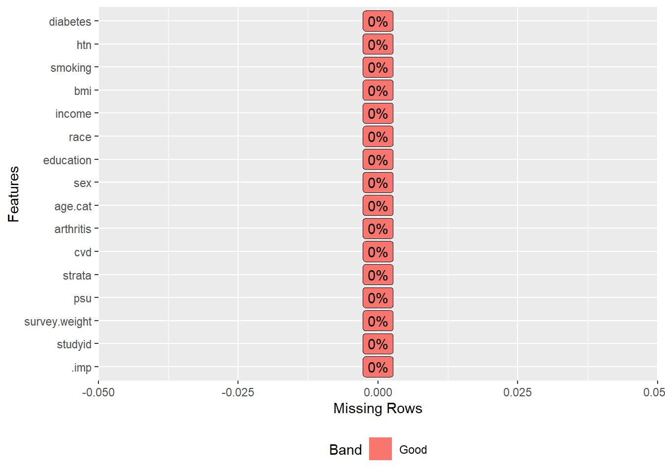
Step 2: PS weighting steps 1-3 by DuGoff et al. (2014)
Our next step is to use steps 1-3 of the PS weighting analysis:
- Step 2.1: Fit the PS model by considering survey features as covariates.
- Step 2.2: Calculate PS weights
- Step 2.3: Balance checking using SMD. Consider SMD <0.2 as a good covariate balancing.
Step 2.1: PS model specification
Step 2.2: Estimating PS and calculating weights
dat.ps <- list(NULL)

m <- 5 # 5 imputed dataset

# PS weighting on each of the imputed datasets
for (ii in 1:m) {
  # Imputed dataset
  dat.imputed <- subset(impdata, .imp == ii)

  # Propensity scores
  ps.fit <- glm(ps.formula, data = dat.imputed, family = binomial("logit"))
  dat.imputed$ps <- fitted(ps.fit)

  # Stabilized weight
  dat.imputed$sweight <- with(dat.imputed,
                              ifelse(I(arthritis == "Rheumatoid arthritis"),
                                     mean(I(arthritis == "Rheumatoid arthritis"))/ps,
                                     (1-mean(I(arthritis == "Rheumatoid arthritis")))/(1-ps)))

  # Dataset
  dat.ps[[ii]] <- dat.imputed
}

# Weight summary
purrr::map_df(dat.ps, function(df){summary(df$sweight)})Step 2.3: Balance checking for each imputed dataset
Now we will check balance in terms of SMD on each dataset.
tab1m <- list(NULL)
for (ii in 1:m) {
  # PS weighted imputed data
  dat <- dat.ps[[ii]]

  # Covariates
  vars <- c("age.cat", "sex", "education", "race", "income", "bmi", "smoking",
            "htn", "diabetes")

  # Design with truncated stabilized weight
  wdesign <- svydesign(ids = ~studyid, weights = ~sweight, data = dat)

  # Balance checking
  tab1m[[ii]] <- svyCreateTableOne(vars = vars, strata = "arthritis", data = wdesign,
                                   test = F)
}
print(tab1m, smd = TRUE)
#> [[1]]
#>                               Stratified by arthritis
#>                                No arthritis    Rheumatoid arthritis SMD
#>   n                             3856.0          316.3
#>   age.cat (%)                                                        0.077
#>      20-49                      2096.4 (54.4)   159.8 (50.5)
#>      50-64                      1010.5 (26.2)    89.2 (28.2)
#>      65+                         749.1 (19.4)    67.3 (21.3)
#>   sex = Female (%)              1900.0 (49.3)   144.1 (45.6)         0.075
#>   education (%)                                                      0.053
#>      Less than high school       764.6 (19.8)    60.9 (19.3)
#>      High school                2109.7 (54.7)   180.9 (57.2)
#>      College graduate or above   981.8 (25.5)    74.4 (23.5)
#>   race (%)                                                           0.074
#>      White                      1173.6 (30.4)   107.0 (33.8)
#>      Black                       917.9 (23.8)    70.1 (22.2)
#>      Hispanic                    933.5 (24.2)    73.4 (23.2)
#>      Others                      831.0 (21.6)    65.8 (20.8)
#>   income (%)                                                         0.045
#>      less than $20,000           685.9 (17.8)    59.3 (18.7)
#>      $20,000 to $74,999         2015.6 (52.3)   158.2 (50.0)
#>      $75,000 and Over           1154.5 (29.9)    98.8 (31.3)
#>   bmi (mean (SD))                29.34 (7.29)   29.93 (6.90)         0.082
#>   smoking (%)                                                        0.211
#>      Never smoker               2362.5 (61.3)   162.7 (51.4)
#>      Previous smoker             814.5 (21.1)    91.9 (29.1)
#>      Current smoker              679.1 (17.6)    61.6 (19.5)
#>   htn = Yes (%)                 2403.5 (62.3)   211.4 (66.8)         0.094
#>   diabetes = Yes (%)             523.3 (13.6)    50.9 (16.1)         0.071
#>
#> [[2]]
#>                               Stratified by arthritis
#>                                No arthritis    Rheumatoid arthritis SMD
#>   n                             3855.7          317.6
#>   age.cat (%)                                                        0.079
#>      20-49                      2096.4 (54.4)   160.2 (50.4)
#>      50-64                      1010.3 (26.2)    89.8 (28.3)
#>      65+                         749.0 (19.4)    67.6 (21.3)
#>   sex = Female (%)              1899.4 (49.3)   144.0 (45.3)         0.079
#>   education (%)                                                      0.050
#>      Less than high school       765.1 (19.8)    61.3 (19.3)
#>      High school                2113.3 (54.8)   181.6 (57.2)
#>      College graduate or above   977.2 (25.3)    74.7 (23.5)
#>   race (%)                                                           0.076
#>      White                      1173.6 (30.4)   107.8 (33.9)
#>      Black                       917.9 (23.8)    71.0 (22.4)
#>      Hispanic                    933.2 (24.2)    72.0 (22.7)
#>      Others                      831.0 (21.6)    66.8 (21.0)
#>   income (%)                                                         0.039
#>      less than $20,000           688.0 (17.8)    57.8 (18.2)
#>      $20,000 to $74,999         2015.9 (52.3)   160.1 (50.4)
#>      $75,000 and Over           1151.8 (29.9)    99.7 (31.4)
#>   bmi (mean (SD))                29.33 (7.22)   29.90 (6.95)         0.081
#>   smoking (%)                                                        0.213
#>      Never smoker               2362.4 (61.3)   162.6 (51.2)
#>      Previous smoker             813.9 (21.1)    91.7 (28.9)
#>      Current smoker              679.3 (17.6)    63.3 (19.9)
#>   htn = Yes (%)                 2394.0 (62.1)   213.6 (67.3)         0.108
#>   diabetes = Yes (%)             522.8 (13.6)    50.3 (15.8)         0.065
#>
#> [[3]]
#>                               Stratified by arthritis
#>                                No arthritis    Rheumatoid arthritis SMD
#>   n                             3856.6          313.7
#>   age.cat (%)                                                        0.088
#>      20-49                      2096.4 (54.4)   156.9 (50.0)
#>      50-64                      1010.1 (26.2)    88.9 (28.3)
#>      65+                         750.1 (19.4)    67.9 (21.6)
#>   sex = Female (%)              1900.1 (49.3)   142.2 (45.3)         0.079
#>   education (%)                                                      0.069
#>      Less than high school       765.0 (19.8)    57.8 (18.4)
#>      High school                2112.6 (54.8)   182.5 (58.2)
#>      College graduate or above   979.0 (25.4)    73.4 (23.4)
#>   race (%)                                                           0.082
#>      White                      1174.1 (30.4)   106.8 (34.1)
#>      Black                       918.2 (23.8)    69.9 (22.3)
#>      Hispanic                    933.4 (24.2)    69.8 (22.2)
#>      Others                      830.9 (21.5)    67.2 (21.4)
#>   income (%)                                                         0.095
#>      less than $20,000           698.8 (18.1)    63.2 (20.1)
#>      $20,000 to $74,999         2003.2 (51.9)   148.1 (47.2)
#>      $75,000 and Over           1154.6 (29.9)   102.4 (32.7)
#>   bmi (mean (SD))                29.29 (7.21)   29.80 (6.97)         0.072
#>   smoking (%)                                                        0.216
#>      Never smoker               2362.7 (61.3)   160.3 (51.1)
#>      Previous smoker             814.6 (21.1)    91.0 (29.0)
#>      Current smoker              679.2 (17.6)    62.5 (19.9)
#>   htn = Yes (%)                 2398.6 (62.2)   206.3 (65.8)         0.074
#>   diabetes = Yes (%)             523.7 (13.6)    50.9 (16.2)         0.075
#>
#> [[4]]
#>                               Stratified by arthritis
#>                                No arthritis    Rheumatoid arthritis SMD
#>   n                             3856.2          312.9
#>   age.cat (%)                                                        0.098
#>      20-49                      2096.3 (54.4)   154.7 (49.5)
#>      50-64                      1010.8 (26.2)    91.2 (29.1)
#>      65+                         749.1 (19.4)    67.0 (21.4)
#>   sex = Female (%)              1900.1 (49.3)   144.4 (46.2)         0.063
#>   education (%)                                                      0.064
#>      Less than high school       763.7 (19.8)    58.4 (18.7)
#>      High school                2115.2 (54.9)   181.5 (58.0)
#>      College graduate or above   977.2 (25.3)    72.9 (23.3)
#>   race (%)                                                           0.078
#>      White                      1173.7 (30.4)   106.5 (34.0)
#>      Black                       918.0 (23.8)    70.1 (22.4)
#>      Hispanic                    933.5 (24.2)    71.2 (22.8)
#>      Others                      831.0 (21.5)    65.0 (20.8)
#>   income (%)                                                         0.096
#>      less than $20,000           694.1 (18.0)    63.9 (20.4)
#>      $20,000 to $74,999         2009.3 (52.1)   148.3 (47.4)
#>      $75,000 and Over           1152.9 (29.9)   100.7 (32.2)
#>   bmi (mean (SD))                29.28 (7.21)   29.86 (7.13)         0.081
#>   smoking (%)                                                        0.209
#>      Never smoker               2362.7 (61.3)   161.3 (51.6)
#>      Previous smoker             813.8 (21.1)    90.7 (29.0)
#>      Current smoker              679.7 (17.6)    60.9 (19.5)
#>   htn = Yes (%)                 2394.5 (62.1)   206.6 (66.0)         0.082
#>   diabetes = Yes (%)             523.0 (13.6)    50.2 (16.0)         0.069
#>
#> [[5]]
#>                               Stratified by arthritis
#>                                No arthritis    Rheumatoid arthritis SMD
#>   n                             3855.7          316.8
#>   age.cat (%)                                                        0.080
#>      20-49                      2096.4 (54.4)   159.6 (50.4)
#>      50-64                      1010.3 (26.2)    89.8 (28.4)
#>      65+                         749.1 (19.4)    67.4 (21.3)
#>   sex = Female (%)              1899.6 (49.3)   143.9 (45.4)         0.077
#>   education (%)                                                      0.060
#>      Less than high school       767.4 (19.9)    62.1 (19.6)
#>      High school                2110.3 (54.7)   181.8 (57.4)
#>      College graduate or above   978.0 (25.4)    72.9 (23.0)
#>   race (%)                                                           0.074
#>      White                      1173.5 (30.4)   107.1 (33.8)
#>      Black                       917.9 (23.8)    70.1 (22.1)
#>      Hispanic                    933.4 (24.2)    73.1 (23.1)
#>      Others                      830.9 (21.5)    66.5 (21.0)
#>   income (%)                                                         0.047
#>      less than $20,000           685.0 (17.8)    60.6 (19.1)
#>      $20,000 to $74,999         2022.6 (52.5)   159.2 (50.3)
#>      $75,000 and Over           1148.1 (29.8)    97.0 (30.6)
#>   bmi (mean (SD))                29.31 (7.20)   29.77 (7.04)         0.064
#>   smoking (%)                                                        0.206
#>      Never smoker               2362.7 (61.3)   163.1 (51.5)
#>      Previous smoker             813.3 (21.1)    90.0 (28.4)
#>      Current smoker              679.7 (17.6)    63.6 (20.1)
#>   htn = Yes (%)                 2409.4 (62.5)   210.2 (66.3)         0.080
#>   diabetes = Yes (%)             522.5 (13.6)    50.3 (15.9)         0.066
For each of the datasets, all SMDs except for smoking are less than our specified cut-point of 0.2. We will adjust our outcome model for smoking.
Step 3: Outcome modelling
Our next step is to fit the outcome model on each of the imputed dataset. Note that, we must utilize survey features to correctly estimate the standard error. For this step, we will multiply PS weight and survey weight and create a new weight variable.
3.1 Calculating new weights
3.2 Preparing dataset for ineligible subjects
Now we will add the ineligible subjects(ineligible by study restriction) with the PS weighted datasets, so that we can set up the survey design on the full dataset and then subset the design.
Let us subset the data for ineligible subjects:
# Subset for ineligible
dat.ineligible <- list(NULL)

for(ii in 1:m){
  # Matched dataset
  dat <- dat.ps[[ii]]

  # Create an indicator variable in the full dataset
  dat.full$ineligible <- 1
  dat.full$ineligible[dat.full$studyid %in% dat$studyid] <- 0

  # Subset for ineligible
  dat.ineligible[[ii]] <- subset(dat.full, ineligible == 1)

  # Create the .imp variable on each dataset with .imp 1 to m = 5
  dat.ineligible[[ii]]$.imp <- ii
}

# Dimension of each dataset
lapply(dat.ineligible, dim)
#> [[1]]
#> [1] 5063   19
#>
#> [[2]]
#> [1] 5063   19
#>
#> [[3]]
#> [1] 5063   19
#>
#> [[4]]
#> [1] 5063   19
#>
#> [[5]]
#> [1] 5063   19
The next step is combining matched and ineligible datasets. Before merging, we must ensure the variable names are the same.
# Variables in the matched datasets
names(dat.ps2[[3]])
#>  [1] "studyid"       "survey.weight" "psu"           "strata"
#>  [5] "cvd"           "arthritis"     "age.cat"       "sex"
#>  [9] "education"     "race"          "income"        "bmi"
#> [13] "smoking"       "htn"           "diabetes"      ".imp"
#> [17] "ps"            "sweight"       "new_weight"

# Variables in the ineligible datasets
names(dat.ineligible[[3]])
#>  [1] "studyid"       "survey.weight" "psu"           "strata"
#>  [5] "cvd"           "rheumatoid"    "age"           "sex"
#>  [9] "education"     "race"          "income"        "bmi"
#> [13] "smoking"       "htn"           "diabetes"      "age.cat"
#> [17] "arthritis"     "ineligible"    ".imp"
dat.ineligible2 <- list(NULL)
for (ii in 1:m) {
dat <- dat.ineligible[[ii]]
# Drop the ineligible variable from the dataset
dat$ineligible <- NULL
# Create ps and sweight
dat$ps <- NA
dat$sweight <- NA
dat$new_weight <- NA
# Keep only those variables available in the matched dataset
vars <- names(dat.ps2[[1]])
dat <- dat[,vars]
# Ineligible datasets in list format
dat.ineligible2[[ii]] <- dat
}3.2 Combining eligible (imputed and PS weighted) and ineligible (unimputed) subjects
Now, we will merge imputed eligible and unimputed ineligible subjects. We should have m = 5 copies of the full dataset with 9,254 subjects on each.
dat.full2 <- list(NULL)

for (ii in 1:m) {
  # Eligible
  d1 <- data.frame(dat.ps2[[ii]])
  d1$eligible <- 1

  # Ineligible
  d2 <- data.frame(dat.ineligible2[[ii]])
  d2$eligible <- 0

  # Full data
  d3 <- rbind(d1, d2)

  #  New weight variable in the full dataset
  d3$new_weight <- 0
  d3$new_weight[d3$studyid %in% d1$studyid] <- d1$new_weight

  # Full data in list format
  dat.full2[[ii]] <- d3
}
lapply(dat.full2, dim)
#> [[1]]
#> [1] 9254   20
#>
#> [[2]]
#> [1] 9254   20
#>
#> [[3]]
#> [1] 9254   20
#>
#> [[4]]
#> [1] 9254   20
#>
#> [[5]]
#> [1] 9254   20

# Stacked dataset
dat.stacked <- rbindlist(dat.full2)
dim(dat.stacked)
#> [1] 46270    20
3.3 Prepating Survey design and subpopulation of eligible
The next step is to create the design on the combined dataset. Make sure to use the new weight variable that combines survey weights and PS weights.
We can see the length of the subsetted design:
Now we will run the design-adjusted logistic regression, adjusting for smoking since smoking was not balanced in terms of SMD.
Step 3.4: Design adjusted regression analysis
# Design-adjusted logistic regression
fit <- with(w.design, svyglm(I(cvd == "Yes") ~ arthritis + smoking, family = quasibinomial))
res <- exp(as.data.frame(cbind(coef(fit[[1]]),
                               coef(fit[[2]]),
                               coef(fit[[3]]),
                               coef(fit[[4]]),
                               coef(fit[[5]]))))
names(res) <- paste("OR from m =", 1:m)
round(t(res),2)
#>               (Intercept) arthritisRheumatoid arthritis smokingPrevious smoker
#> OR from m = 1        0.04                          1.21                   2.93
#> OR from m = 2        0.04                          1.24                   2.93
#> OR from m = 3        0.04                          1.23                   2.93
#> OR from m = 4        0.04                          1.22                   2.92
#> OR from m = 5        0.04                          1.22                   2.92
#>               smokingCurrent smoker
#> OR from m = 1                  1.55
#> OR from m = 2                  1.56
#> OR from m = 3                  1.54
#> OR from m = 4                  1.55
#> OR from m = 5                  1.55
Step 3.5: Pooling estimates
Now, we will pool the estimate using Rubin’s rule:
Double adjustment
# Outcome model with covariates adjustment
fit2 <- with(w.design, svyglm(I(cvd == "Yes") ~ arthritis + age.cat + sex + education +
                               race + income + bmi + smoking + htn + diabetes,
                             family = quasibinomial))

# Pooled estimate
pooled.estimates <- MIcombine(fit2)
OR <- round(exp(pooled.estimates$coefficients), 2)
OR <- as.data.frame(OR)
CI <- round(exp(confint(pooled.estimates)), 2)
OR <- cbind(OR, CI)
OR