CCHS: Performance
The tutorial outlines the process for evaluating the performance of logistic regression models fitted to complex survey data using R. It focuses on two major aspects: creating Receiver Operating Characteristic (ROC) curves and conducting Archer and Lemeshow Goodness of Fit tests. Here AUC is a measure to evaluate the predictive accuracy of the model, and Archer and Lemeshow test is a statistical test to evaluate how well your model fits the observed data.
See an updated version of this tutorial here that uses svyTable1 package on an NHANES data analysis.
We start by importing the required R packages.
Load data
It loads two datasets from the specified paths.
Three different logistic regression models are fitted to the data:
- Simple model: Model with only OA as a predictor
- Basic model: Model with OA, age and sex
- Complex model: Model with many predictors and some interaction terms
# Formula for Simple model
simple.model <- as.formula(I(CVD=="event") ~ OA)
simple.model
#> I(CVD == "event") ~ OA

# Formula for Basic model
basic.model
#> I(CVD == "event") ~ OA + age + sex
#> attr(,"variables")
#> list(I(CVD == "event"), OA, age, sex)
#> attr(,"factors")
#>                   OA age sex
#> I(CVD == "event")  0   0   0
#> OA                 1   0   0
#> age                0   1   0
#> sex                0   0   1
#> attr(,"term.labels")
#> [1] "OA"  "age" "sex"
#> attr(,"order")
#> [1] 1 1 1
#> attr(,"intercept")
#> [1] 1
#> attr(,"response")
#> [1] 1
#> attr(,".Environment")
#> <environment: R_GlobalEnv>
#> attr(,"predvars")
#> list(I(CVD == "event"), OA, age, sex)
#> attr(,"dataClasses")
#> I(CVD == "event")                OA               age               sex
#>         "logical"          "factor"          "factor"          "factor"
#>         (weights)
#>         "numeric"

# Formula for the Complex model with interactions
aic.int.model
#> I(CVD == "event") ~ OA + age + sex + married + race + edu + income +
#>     bmi + phyact + fruit + bp + diab + doctor + stress + smoke +
#> drink + age:sex + bmi:diablibrary(survey)
# Simple model
fit0 <- svyglm(simple.model,
design = w.design,
family = binomial(logit))
#> Warning in eval(family$initialize): non-integer #successes in a binomial glm!
# Basic model
fit5 <- svyglm(basic.model,
design = w.design,
family = binomial(logit))
#> Warning in eval(family$initialize): non-integer #successes in a binomial glm!
# Complex model with interactions
fit9 <- svyglm(aic.int.model,
design = w.design,
family = binomial(logit))
#> Warning in eval(family$initialize): non-integer #successes in a binomial glm!Model performance
ROC curve
This section defines a function, svyROCw, to plot the ROC curves and calculate the area under the curve (AUC). The function can handle both weighted and unweighted survey data.
- The appropriateness of the fitted logistic regression model needs to be examined before it is accepted for use.
- Plotting the pairs of - sensitivities vs - 1-specificities on a scatter plot provides a Receiver Operating Characteristic (ROC) curve.
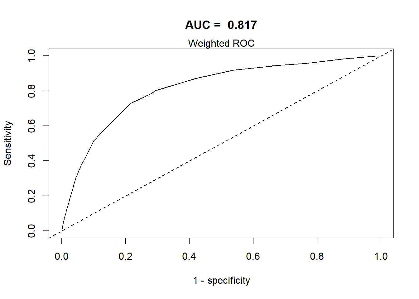
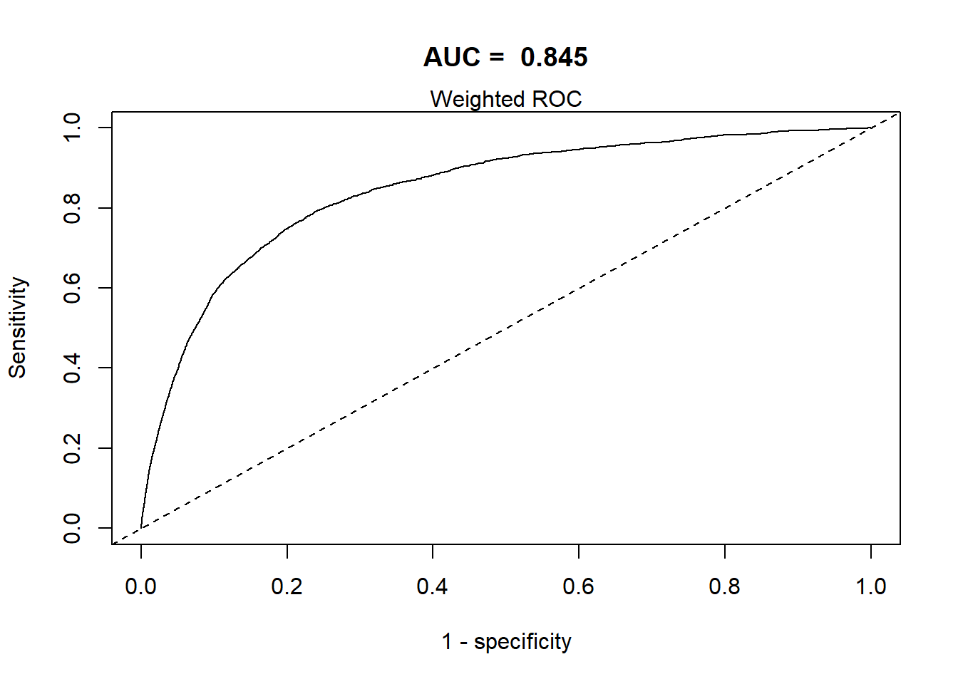
- The area under the ROC curve = AUC / C-statistic.
- ROC/AUC should consider weights for complex surveys.
Grading Guidelines for AUC values:
- 0.90-1.0 excellent discrimination (unusual)
- 0.80-0.90 good discrimination
- 0.70-0.80 fair discrimination
- 0.60-0.70 poor discrimination
- 0.50-0.60 failed discrimination
require(ROCR)
# WeightedROC may not be on cran for all R versions
# devtools::install_github("tdhock/WeightedROC")

library(WeightedROC)
svyROCw <- function(fit=fit,outcome=analytic2$CVD=="event", weight = NULL){
  # ROC curve for
  # Survey Data with Logistic Regression
  if (is.null(weight)){ # require(ROCR)
    prob <- predict(fit, type = "response")
  pred <- prediction(as.vector(prob), outcome)
  perf <- performance(pred, "tpr", "fpr")
  auc <- performance(pred, measure = "auc")
  auc <- auc@y.values[[1]]
  roc.data <- data.frame(fpr = unlist(perf@x.values), tpr = unlist(perf@y.values),
      model = "Logistic")
  with(data = roc.data,plot(fpr, tpr, type="l", xlim=c(0,1), ylim=c(0,1), lwd=1,
     xlab="1 - specificity", ylab="Sensitivity",
     main = paste("AUC = ", round(auc,3))))
  mtext("Unweighted ROC")
  abline(0,1, lty=2)
  } else { # library(WeightedROC)
    outcome <- as.numeric(outcome)
  pred <- predict(fit, type = "response")
  tp.fp <- WeightedROC(pred, outcome, weight)
  auc <- WeightedAUC(tp.fp)
  with(data = tp.fp,plot(FPR, TPR, type="l", xlim=c(0,1), ylim=c(0,1), lwd=1,
     xlab="1 - specificity", ylab="Sensitivity",
     main = paste("AUC = ", round(auc,3))))
  abline(0,1, lty=2)
  mtext("Weighted ROC")
  }
}summary(analytic2$weight)
#> Min. 1st Qu. Median Mean 3rd Qu. Max.
#> 1.17 71.56 137.95 214.61 261.91 7154.95
analytic2$corrected.weight <- weights(w.design)
summary(analytic2$corrected.weight)
#> Min. 1st Qu. Median Mean 3rd Qu. Max.
#> 0.39 23.85 45.98 71.54 87.30 2384.98
svyROCw(fit=fit0,outcome=analytic2$CVD=="event", weight = analytic2$corrected.weight)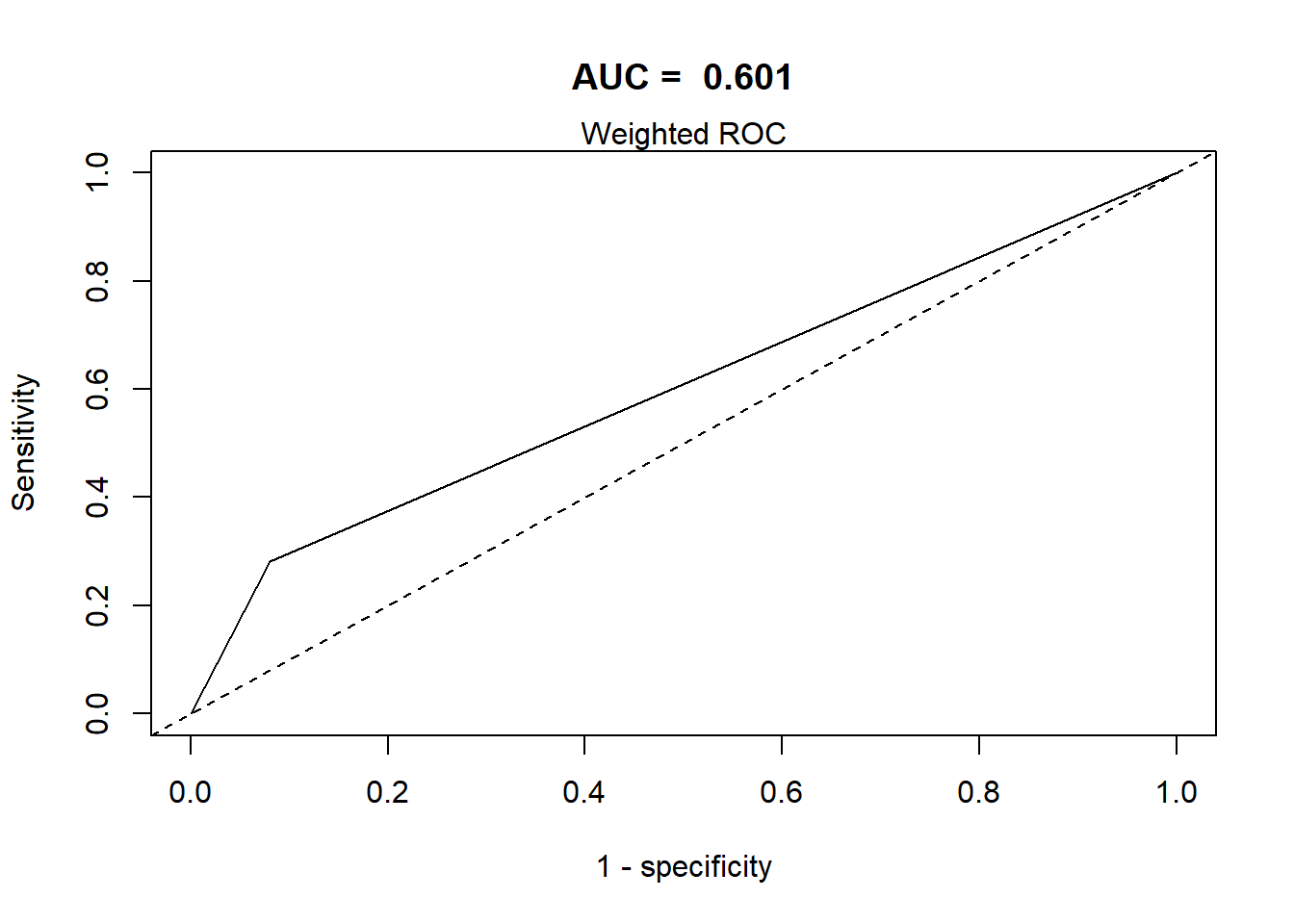
svyROCw (and AL.gof below) incorporate only the survey weights (id = ~1); they do not account for stratification or clustering. The resulting weighted AUC and Archer-Lemeshow test are therefore design-aware only with respect to weighting. For a fully design-correct analysis that also uses strata and PSU/cluster information, use the AL.gof2 function shown later in this tutorial, or see the updated NHANES tutorial.
Archer and Lemeshow test
This test helps to evaluate how well the model fits the data. A Goodness of Fit (GOF) function AL.gof is defined. If the p-value from this test is greater than a certain threshold (e.g., 0.05), the model fit is considered acceptable.
- Hosmer Lemeshow-type tests are most useful as a very crude way to screen for fit problems, and should not be taken as a definitive diagnostic of a ‘good’ fit.
- problem in small sample size
- Dependent on G (group)
- Archer and Lemeshow (2006) extended the standard Hosmer and Lemeshow GOF test for complex surveys.
- After fitting the survey weighted logistic regression, the F-adjusted mean residual goodness-of-fit test could suggest
- no evidence of lack of fit (if P-value > a reasonable cut-point, e.g., 0.05)
- evidence of lack of fit (if P-value < a reasonable cut-point, e.g., 0.05)
AL.gof <- function(fit=fit, data = analytic2,
                   weight = "corrected.weight"){
  # Archer-Lemeshow Goodness of Fit Test for
  # Survey Data with Logistic Regression
  r <- residuals(fit, type="response")
  f<-fitted(fit)
  breaks.g <- c(-Inf, quantile(f,  (1:9)/10), Inf)
  breaks.g <- breaks.g + seq_along(breaks.g) * .Machine$double.eps
  g<- cut(f, breaks.g)
  data2g <- cbind(data,r,g)
  newdesign <- svydesign(id=~1,
                         weights=as.formula(paste0("~",weight)),
                        data=data2g)
  decilemodel<- svyglm(r~g, design=newdesign)
  res <- regTermTest(decilemodel, ~g)
  return(res)
}AL.gof(fit0, analytic2, weight ="corrected.weight")
#> Wald test for g
#> in svyglm(formula = r ~ g, design = newdesign)
#> F = 2.20807e-22 on 1 and 185611 df: p= 1
AL.gof(fit5, analytic2, weight ="corrected.weight")
#> Wald test for g
#> in svyglm(formula = r ~ g, design = newdesign)
#> F = 2.795204 on 8 and 185604 df: p= 0.0042898
AL.gof(fit9, analytic2, weight = "corrected.weight")
#> Wald test for g
#> in svyglm(formula = r ~ g, design = newdesign)
#> F = 2.650332 on 9 and 185603 df: p= 0.0045417Additional function
If the survey data contains strata and cluster, then the following function will be useful:
AL.gof2 <- function(fit=fit7, data = analytic,
                   weight = "corrected.weight", psu = "psu", strata= "strata"){
  # Archer-Lemeshow Goodness of Fit Test for
  # Survey Data with Logistic Regression
  r <- residuals(fit, type="response")
  f<-fitted(fit)
  breaks.g <- c(-Inf, quantile(f,  (1:9)/10), Inf)
  breaks.g <- breaks.g + seq_along(breaks.g) * .Machine$double.eps
  g<- cut(f, breaks.g)
  data2g <- cbind(data,r,g)
  newdesign <- svydesign(id=as.formula(paste0("~",psu)),
                         strata=as.formula(paste0("~",strata)),
                         weights=as.formula(paste0("~",weight)),
                        data=data2g, nest = TRUE)
  decilemodel<- svyglm(r~g, design=newdesign)
  res <- regTermTest(decilemodel, ~g)
  return(res)
}
Video content (optional)
For those who prefer a video walkthrough, feel free to watch the video below, which offers a description of an earlier version of the above content.