
Reproducing NHANES results
The section instructs on reproducing the results from a specific article, detailing the eligibility criteria and variables of interest, guiding the user through accessing, merging, and filtering relevant NHANES data, and then recoding and comparing the results to ensure they match with the original article’s findings, all supported with visual aids and R code examples.
Example article
Let us use the article by Flegal et al. (2016) as our reference. DOI:10.1001/jama.2016.6458.
Flegal et al. (2016)
Task
Objectives are to
- Learn how to download and select pertinent NHANES data
- Understand the importance of cleaning and transforming the data
- Reproduce findings from an existing research paper using NHANES data
Our specific task in this tutorial is to reproduce the numbers reported in Table 1 from this article.
Eligibility criteria
Methods section from this article says:
- “For adults aged 20 years or older, obesity was defined according to clinical guidelines.”
- “Pregnant women were excluded from analysis.”
- “Participant age was grouped into categories of 20 to 39 years, 40 to 59 years, and 60 years and older.”
- Table 1 title says NHANES 2013-2014 was used.
Variables of interest
Before diving into NHANES, take some time to comprehend its structure. Detailed documentation provides crucial information about variables, age categories, and other specifics.
Variables of interest:
-
age(eligibility and stratifying variable) -
sex(stratifying variable) -
race(stratifying variable) -
pregnancy status(eligibility) -
obesity/BMI status(main variable of interest for the paper)
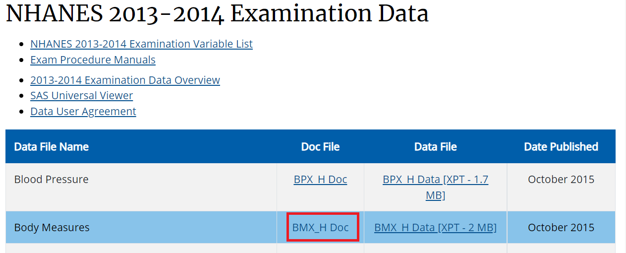
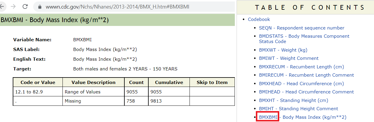
Searching for necessary variables
Search these variables using the NHANES variable keyword search within the 2013-14 cycle: cdc.gov/nchs/nhanes/search/
- Below is an example for BMI variable search:
- Identifying the component: Note that H is the index for 2013-14 cycle as seen in the picture:
- Identifying the variable:
- Rest of the variables all coming from demographic component

Downloading relevant variables
You can download NHANES data directly from their website or use a package that allows easy access to NHANES data sets. For this tutorial, we’ll be downloading data specifically from the 2013-2014 cycle, focusing on demographics and BMI metrics.
NHANES data often comes coded numerically for various categories, making it less straightforward to understand. Use the available translation functions to convert these codes into meaningful categories, easing the data interpretation process.
Demographic data
For the demographic data, we will use the DEMO_H file, where the index H represents the 2013-14 cycle.
Index H represents NHANES 2013-14 cycle
Tip
We use the nhanes function to download a NHANES datafile and nhanesTranslate function to encode the categorical variables to match with the CDC website.
library(nhanesA)
demo13 <- nhanes('DEMO_H')
Demo13 <- nhanesTranslate('DEMO_H', names(demo13), data=demo13)
#> Translated columns: SDDSRVYR RIDSTATR RIAGENDR RIDRETH1 RIDRETH3 RIDEXMON DMQMILIZ DMQADFC DMDBORN4 DMDCITZN DMDYRSUS DMDEDUC3 DMDEDUC2 DMDMARTL RIDEXPRG SIALANG SIAPROXY SIAINTRP FIALANG FIAPROXY FIAINTRP MIALANG MIAPROXY MIAINTRP AIALANGA DMDHHSIZ DMDFMSIZ DMDHHSZA DMDHHSZB DMDHHSZE DMDHRGND DMDHRBR4 DMDHREDU DMDHRMAR DMDHSEDU INDHHIN2 INDFMIN2
Examination data
We are using same H index for BMI.
See all the column names in the data
names(Demo13)
#>  [1] "SEQN"     "SDDSRVYR" "RIDSTATR" "RIAGENDR" "RIDAGEYR" "RIDAGEMN"
#>  [7] "RIDRETH1" "RIDRETH3" "RIDEXMON" "RIDEXAGM" "DMQMILIZ" "DMQADFC"
#> [13] "DMDBORN4" "DMDCITZN" "DMDYRSUS" "DMDEDUC3" "DMDEDUC2" "DMDMARTL"
#> [19] "RIDEXPRG" "SIALANG"  "SIAPROXY" "SIAINTRP" "FIALANG"  "FIAPROXY"
#> [25] "FIAINTRP" "MIALANG"  "MIAPROXY" "MIAINTRP" "AIALANGA" "DMDHHSIZ"
#> [31] "DMDFMSIZ" "DMDHHSZA" "DMDHHSZB" "DMDHHSZE" "DMDHRGND" "DMDHRAGE"
#> [37] "DMDHRBR4" "DMDHREDU" "DMDHRMAR" "DMDHSEDU" "WTINT2YR" "WTMEC2YR"
#> [43] "SDMVPSU"  "SDMVSTRA" "INDHHIN2" "INDFMIN2" "INDFMPIR"
names(Exam13)
#>  [1] "SEQN"     "BMDSTATS" "BMXWT"    "BMIWT"    "BMXRECUM" "BMIRECUM"
#>  [7] "BMXHEAD"  "BMIHEAD"  "BMXHT"    "BMIHT"    "BMXBMI"   "BMDBMIC"
#> [13] "BMXLEG"   "BMILEG"   "BMXARML"  "BMIARML"  "BMXARMC"  "BMIARMC"
#> [19] "BMXWAIST" "BMIWAIST" "BMXSAD1"  "BMXSAD2"  "BMXSAD3"  "BMXSAD4"
#> [25] "BMDAVSAD" "BMDSADCM"
Retain only useful variables
Quick look at the data
Merge data
You might find that the demographic data and BMI data are in separate files. In that case, you’ll need to combine them using a common ID variable. Make sure the data aligns correctly during this process.
Use the ID variable SEQN to merge both data:
Within NHANES datasets in a given cycle, each person has an unique identifier number (variable name SEQN). We can use this SEQN variable to merge their data.
Investigate merged data
Let’s check whether any missing data available.
require(tableone)
#> Loading required package: tableone
tab_nhanes <- CreateTableOne(data=merged.data, includeNA = TRUE)
print(tab_nhanes, showAllLevels = TRUE)
#>
#>                        level
#>   n
#>   RIDEXPRG (%)         Yes, positive lab pregnancy test or self-reported pregnant at exam
#>                        The participant was not pregnant at exam
#>                        Cannot ascertain if the participant is pregnant at exam
#>                        <NA>
#>   RIAGENDR (%)         Male
#>                        Female
#>   RIDAGEYR (mean (SD))
#>   RIDRETH3 (%)         Mexican American
#>                        Other Hispanic
#>                        Non-Hispanic White
#>                        Non-Hispanic Black
#>                        Non-Hispanic Asian
#>                        Other Race - Including Multi-Racial
#>   BMXBMI (mean (SD))
#>
#>                        Overall
#>   n                    10175
#>   RIDEXPRG (%)            65 ( 0.6)
#>                         1150 (11.3)
#>                           94 ( 0.9)
#>                         8866 (87.1)
#>   RIAGENDR (%)          5003 (49.2)
#>                         5172 (50.8)
#>   RIDAGEYR (mean (SD)) 31.48 (24.42)
#>   RIDRETH3 (%)          1730 (17.0)
#>                          960 ( 9.4)
#>                         3674 (36.1)
#>                         2267 (22.3)
#>                         1074 (10.6)
#>                          470 ( 4.6)
#>   BMXBMI (mean (SD))   25.68 (7.96)
As we can see, the RIDEXPRG variable contains a huge amount of missing information.
BMI also contains many missing values.
Applying eligibility criteria
We subset the data using criteria similar to the JAMA paper by Flegal et al. (2016) (see above)
Flegal et al. (2016)
# No missing BMI
analytic.data1 <- subset(merged.data, !is.na(BMXBMI))
dim(analytic.data1)
#> [1] 9055    5

# Age >= 20
analytic.data2 <- subset(analytic.data1, RIDAGEYR >= 20)
dim(analytic.data2)
#> [1] 5520    5


table(analytic.data2$RIDEXPRG,useNA = "always")
#>
#> Yes, positive lab pregnancy test or self-reported pregnant at exam
#>                                                                 65
#>                           The participant was not pregnant at exam
#>                                                               1143
#>            Cannot ascertain if the participant is pregnant at exam
#>                                                                 44
#>                                                               <NA>
#>                                                               4268
# Pregnant women excluded
analytic.data3 <-
  subset(analytic.data2, is.na(RIDEXPRG) |
           RIDEXPRG != "Yes, positive lab pregnancy test")
dim(analytic.data3)
#> [1] 5520    5
Note
This exclusion keys on the exact translated factor label "Yes, positive lab pregnancy test", so it is sensitive to any future change in the nhanesA translation labels; before relying on it, confirm the available levels (e.g., run table(analytic.data2$RIDEXPRG, useNA = "always") as shown above), or filter on the numeric code (RIDEXPRG == 1) prior to translation. Records with RIDEXPRG missing (NA) or coded as “cannot ascertain” are intentionally retained, since pregnancy status could not be confirmed positive for them. With the current labels the row count drops from 5520 to 5455, matching the eligible sample.
Recoding variables
Recode similar to the JAMA paper by Flegal et al. (2016) (see above)
Flegal et al. (2016)
analytic.data3$AgeCat <- cut(analytic.data3$RIDAGEYR,
                           c(0,20,40,60,Inf),
                           right = FALSE)
analytic.data3$Gender <- car::recode(analytic.data3$RIAGENDR,
                                "'1'='Male'; '2'='Female'")
table(analytic.data3$Gender,useNA = "always")
#>
#> Female   Male   <NA>
#>   2882   2638      0
analytic.data3$Race <- car::recode(analytic.data3$RIDRETH3,
                                "c('Mexican American',
                                'Other Hispanic')='Hispanic';
                                'Non-Hispanic White'='White';
                                'Non-Hispanic Black'='Black';
                                'Non-Hispanic Asian'='Asian';
                                else=NA")
analytic.data3$Race <-
  factor(analytic.data3$Race,
         levels = c('White', 'Black', 'Asian', 'Hispanic'))
Reproducing Table 1
Cross-reference the variable names with the NHANES data dictionary to ensure they align with your research questions.
Let’s now compare our table with with the Table 1 in the article:
# Dataset for males
analytic.data3m <- subset(analytic.data3, Gender == "Male")

## Dataset for females
analytic.data3f <- subset(analytic.data3,  Gender == "Female")

# Frequency table by age and gender
with(analytic.data3, table(AgeCat,Gender))
#>           Gender
#> AgeCat     Female Male
#>   [0,20)        0    0
#>   [20,40)     963  909
#>   [40,60)    1002  897
#>   [60,Inf)    917  832
apply(with(analytic.data3, table(AgeCat,Gender)),1,sum)
#>   [0,20)  [20,40)  [40,60) [60,Inf)
#>        0     1872     1899     1749

# Frequency table by age and race
with(analytic.data3, table(AgeCat,Race))
#>           Race
#> AgeCat     White Black Asian Hispanic
#>   [0,20)       0     0     0        0
#>   [20,40)    756   381   222      423
#>   [40,60)    760   384   252      449
#>   [60,Inf)   850   370   156      353

# Frequency table by age and race for males
with(analytic.data3m, table(AgeCat,Race))
#>           Race
#> AgeCat     White Black Asian Hispanic
#>   [0,20)       0     0     0        0
#>   [20,40)    386   182   106      189
#>   [40,60)    360   179   120      215
#>   [60,Inf)   384   195    74      169

# Frequency table by age and race for females
with(analytic.data3f, table(AgeCat,Race))
#>           Race
#> AgeCat     White Black Asian Hispanic
#>   [0,20)       0     0     0        0
#>   [20,40)    370   199   116      234
#>   [40,60)    400   205   132      234
#>   [60,Inf)   466   175    82      184
As we can see, our frequencies exactly match with Table 1 in the article.
Also see (Dhana 2023) for a tidyverse solution
Tip
If your research aims to make population-level inferences, ensure that you also download sampling weights, stratum and cluster variables. These aren’t mandatory for basic analysis but are crucial for population-level conclusions. We will explore more about this in the survey data analysis chapter.
References
Dhana, A. 2023. “R & Python for Data Science.” https://datascienceplus.com/.
Flegal, Katherine M, Deanna Kruszon-Moran, Margaret D Carroll, Cheryl D Fryar, and Cynthia L Ogden. 2016. “Trends in Obesity Among Adults in the United States, 2005 to 2014.” Jama 315 (21): 2284–91.