Importing NHIS to R
This tutorial provides instructions on accessing the National Health Interview Survey (NHIS) dataset from the US Centers for Disease Control and Prevention (CDC) website and importing it into the RStudio environment.
NHIS datafile and documents
The NHIS files are stored in the NHIS website in different formats. You can import this data in any statistical package that supports these file formats, e.g., ASCII, CSV, SAS.
In the recent NHIS (2019 or later), data are available in 5 categories:
- Interview data for adults
- Interview data for children
- Imputed income for adults
- Imputed income for children
- Paradata
In the earlier NHIS (before 2019), data are available in 8 categories:
- Family file
- Household file
- Person file
- Child file
- Adult file
- Imputed income
- Functioning and disability
- Paradata
Combining data
Different cycles
It is possible to combine datasets from different years/cycles together in NHIS. Similar to NHANES, identification of the same person in NHIS across different cycles is not possible in the public release datasets. For appending data from different cycles, please make sure that the variable names/labels are the same/identical in years under consideration (in some years, names and labels do change).
Within the same cycle
Within NHIS datasets in a given cycle, each sampled person has a household number (HHX), family number (FMX), and a person number within family (FPX). We can create a unique identifier based on these three variables and merge the datasets.
Accessing NHIS Data
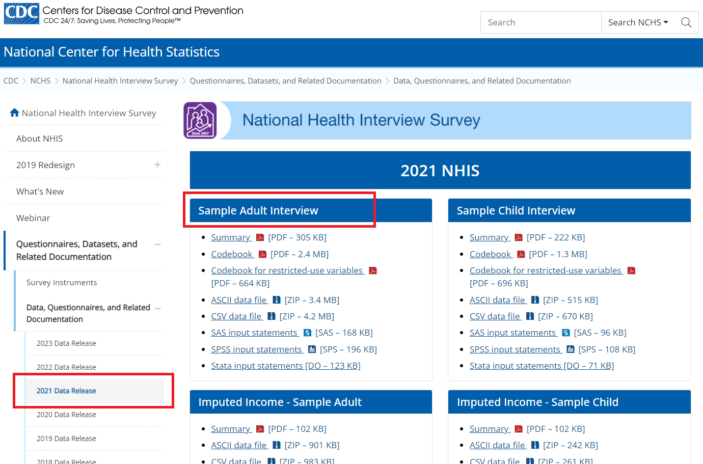
NHIS survey datasets are publicly available at https://www.cdc.gov/nchs/nhis/
Unlike NHANES where a R package is available to download the dataset, NHIS datasets need to be downloaded directly from the CDC website. In the following example, we will see how to download ‘Adult’ data from 2021 NHIS, and check associated variable in that dataset.
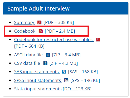
- Step 1: Say, for example, we are interested to download the adult dataset in the CSV format:
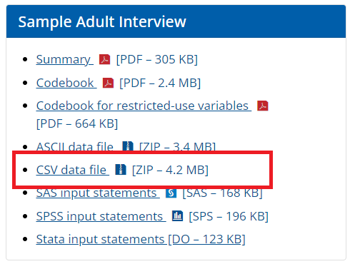
- Step 2: We can download the data in the local PC folder, unzip it, and then read the data into R as as follows:
-
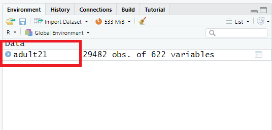
Step 3: Once data is imported in RStudio, we will see the
adult21object listed under data window (see below):
-
Step 4: We can check the variable names in this
adult21dataset using thenamesfunction.
-
Step 5: We can check how many unique adults are in this
adult21dataset. Note that theHHXvariable in the dataset is the unique household identifier, where only one adult per household was selected for interview. We can use thisHHXvariable to merge adult datafile with other datafiles (e.g., child data).
-
Step 6: We can open the data in RStudio in the dataview window (by clicking the
adult21data from the data window). The next Figure shows only a few columns and rows from this large dataset. Note that there are some values marked as “NA”, which represents missing values.
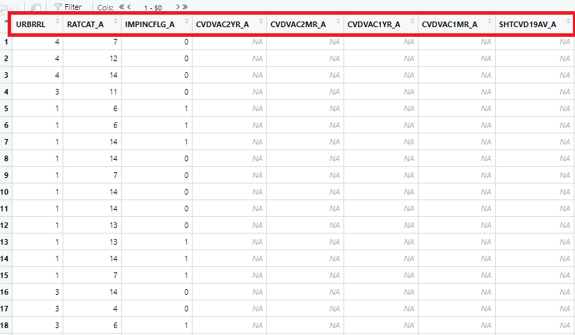
- Step 7: To understand what the column names mean in this Figure, we need to take a look at the codebook, which is also available on the CDC website:
-
Step 8: We can see a check for the column or variables, e.g.,
REGION, in the codebook:
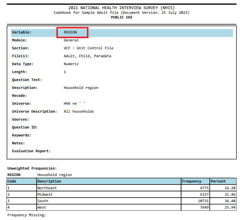
-
Step 9: We can assess if the numbers reported under count matches with what we get from the
adult21data we just imported (particularly, for theREGIONvariable):
Similarly, we can download the child data and open it in R:
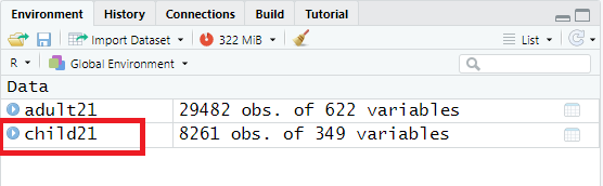
Let’s check how many unique children are in this child21 dataset:
Now let’s check for the column or variables, e.g., SEX_C, in the codebook:
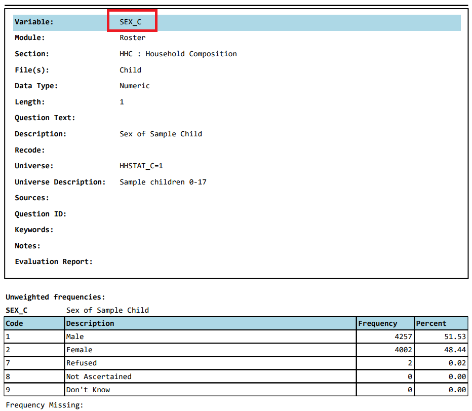
We can assess if the numbers reported under count matches with what we get from the child21 data we just imported:
Merging within the same cycle
Note
We can use HHX variable to merge different datafiles within the same survey cycle.
As mentioned earlier, HHX variable in the dataset is the unique household identifier. We can use this HHX variable to merge different datafiles within the same survey cycle. Say, we are interested in merging child age (AGEP_C) and sex (SEX_C) variables with the adult datafile. We can use the merge function as follows:
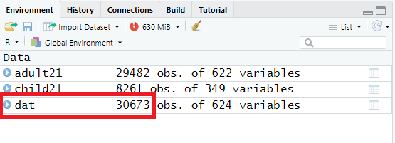
As we can see, there are data from 30,673 unique households, suggesting that not all children are sampled from the same household of sampled adults.
Table 1
Now we will use the adult21 dataset to create Table 1 with utilizing survey features (i.e., psu, strata, and weights). For that, let us create/recode some variables:
In a following chapter about survey data analysis, we will explain what these survey features mean.
# Heart attack
adult21$heart.attack <- car::recode(adult21$MIEV_A, " 2 = 'No'; 1 = 'Yes'; else = NA",
                                levels = c("No", "Yes"), as.factor = T)
table(adult21$heart.attack, useNA = "always")
#>
#>    No   Yes  <NA>
#> 28378  1078    26

# Diabetes
adult21$diabetes <- car::recode(adult21$DIBEV_A, " 2 = 'No'; 1 = 'Yes'; else = NA",
                            levels = c("No", "Yes"), as.factor = T)
table(adult21$diabetes, useNA = "always")
#>
#>    No   Yes  <NA>
#> 26318  3134    30

# Sex
adult21$sex <- car::recode(adult21$SEX_A, " '1'='Male'; '2'='Female'; else=NA",
                       levels = c("Female", "Male"), as.factor = T)
table(adult21$sex, useNA = "always")
#>
#> Female   Male   <NA>
#>  16102  13378      2

# Pseudo-PSU
adult21$psu <- adult21$PPSU
adult21$psu <- as.factor(adult21$psu)
table(adult21$psu, useNA = "always")
#>
#>    1    2    3    4    5    6    7    8    9   10   11   12   13   14   15   16
#> 1952 1599 1141  792  669  461  549  662  629  840  521  359  491  421  405  346
#>   17   18   19   20   21   22   23   24   25   26   27   28   29   30   31   32
#>  156  221  348  531  596  656  588  593  383  647  374  294  218   57  310  334
#>   33   34   35   36   37   38   39   40   41   42   43   44   45   46   47   48
#>  269  369  410  447  180  279  263   85   70  208  175  224  302  270  396  376
#>   49   50   51   52   53   54   55   56   57   58   59   60   61   62   63   64
#>  202  240  303  253  349  249   75   67  257  203  234  327  410  364  252  247
#>   65   66   67   68   72   73   74   75   76   77   78   79   80   81   82   87
#>  199  149   96   22   65   42  108  131   37   41   31   28   50   46   64   31
#>   89   90   91   92   93   97   98   99  100  101  102  103  104  108  109  110
#>   81   28  132  170   64   86   45   32  144  128  129  171  117   63   48   13
#>  114  127  128  134  139  140  150  151  152  153 <NA>
#>   54   44   10   29   69   18   46   50   49   24    0

# Pseudo-stratum
adult21$strata <- adult21$PSTRAT
adult21$strata <- as.factor(adult21$strata)
table(adult21$strata, useNA = "always")
#>
#>  100  101  102  103  104  105  106  107  108  109  110  111  112  113  114  115
#>  736  714  589  480  499  605  733  748  757  629  623  614  158  914  386  603
#>  116  117  118  119  120  121  122  123  124  125  126  127  128  129  130  131
#>  192  678  661  842  549  510  606  306  517  385  633  418  265  801  449  558
#>  132  133  134  135  136  137  138  139  140  141  142  143  144  145  146  147
#>  558  563  434  532  595  576  494  370  644  485  460  738  625  368  412  650
#>  148  149  150  151 <NA>
#>  672  531  556 1061    0

# Sampling weight
adult21$sweight <- adult21$WTFA
summary(adult21$sweight)
#>    Min. 1st Qu.  Median    Mean 3rd Qu.    Max.
#>   793.2  4698.3  7402.6  8586.9 10671.1 71378.0

# Drop the missing values associated with Heart attack, Diabetes, Sex
dat.analytic <- adult21[complete.cases(adult21$heart.attack),]
dat.analytic <- dat.analytic[complete.cases(dat.analytic$diabetes),]
dat.analytic <- dat.analytic[complete.cases(dat.analytic$sex),]
dim(dat.analytic)
#> [1] 29435   628
First, we will create the survey design. Second, we will report Table 1 with heart attack and sex variable, stratified by diabetes.
library(tableone)
library(survey)

# Indicator in the full data
adult21$indicator <- 1
adult21$indicator[adult21$HHX %in% dat.analytic$HHX] <- 0
table(adult21$indicator)
#>
#>     0     1
#> 29435    47

# Survey design
w.design <- svydesign(id = ~psu, strata = ~strata, weights = ~sweight, data = adult21, nest = T)

# Subset
w.design0 <- subset(w.design, indicator == 0)

# Table 1
tab1 <- svyCreateTableOne(var = c("heart.attack", "sex"), strata= "diabetes",
                          data = w.design0, test = FALSE)
print(tab1)
#>                         Stratified by diabetes
#>                          No                  Yes
#>   n                      228524605.2         24325386.4
#>   heart.attack = Yes (%)   5335722.7 ( 2.3)   2358175.6 ( 9.7)
#>   sex = Male (%)         109610086.2 (48.0)  12510287.1 (51.4)
Regression analysis
Let’s run a regression analysis with utilizing survey features.