NHANES: Blood Pressure
The tutorial aims to guide the user through the process of analyzing health survey data, focusing specifically on the relationship between various demographic factors and blood pressure levels.
Required packages are imported for data manipulation and statistical analysis.
Load data
NHANES survey data is loaded into the workspace.
Regression summary
Bivariate Regression
Four separate models are constructed to explore the relationship between blood pressure and individual demographic variables like race, age, gender, and marital status.
summary(fit1r <- glm(blood.pressure ~ race, data=analytic.data))
#>
#> Call:
#> glm(formula = blood.pressure ~ race, data = analytic.data)
#>
#> Coefficients:
#>                        Estimate Std. Error t value Pr(>|t|)
#> (Intercept)             65.4408     0.3566 183.528  < 2e-16 ***
#> raceNon-Hispanic Black   2.1594     0.4891   4.415 1.02e-05 ***
#> raceNon-Hispanic White   0.9957     0.4498   2.214   0.0269 *
#> raceOther Hispanic       0.3422     0.5553   0.616   0.5378
#> raceOther race           3.0601     0.5326   5.746 9.54e-09 ***
#> ---
#> Signif. codes:  0 '***' 0.001 '**' 0.01 '*' 0.05 '.' 0.1 ' ' 1
#>
#> (Dispersion parameter for gaussian family taken to be 168.7193)
#>
#>     Null deviance: 1202625  on 7086  degrees of freedom
#> Residual deviance: 1194870  on 7082  degrees of freedom
#>   (2884 observations deleted due to missingness)
#> AIC: 56463
#>
#> Number of Fisher Scoring iterations: 2summary(fit1a <- glm(blood.pressure ~ age.centred, data=analytic.data))
#>
#> Call:
#> glm(formula = blood.pressure ~ age.centred, data = analytic.data)
#>
#> Coefficients:
#> Estimate Std. Error t value Pr(>|t|)
#> (Intercept) 68.297917 0.158325 431.4 <2e-16 ***
#> age.centred 0.179501 0.006623 27.1 <2e-16 ***
#> ---
#> Signif. codes: 0 '***' 0.001 '**' 0.01 '*' 0.05 '.' 0.1 ' ' 1
#>
#> (Dispersion parameter for gaussian family taken to be 153.7967)
#>
#> Null deviance: 1202625 on 7086 degrees of freedom
#> Residual deviance: 1089649 on 7085 degrees of freedom
#> (2884 observations deleted due to missingness)
#> AIC: 55804
#>
#> Number of Fisher Scoring iterations: 2summary(fit1g <- glm(blood.pressure ~ gender, data=analytic.data))
#>
#> Call:
#> glm(formula = blood.pressure ~ gender, data = analytic.data)
#>
#> Coefficients:
#> Estimate Std. Error t value Pr(>|t|)
#> (Intercept) 67.4863 0.2210 305.409 < 2e-16 ***
#> genderFemale -1.4885 0.3091 -4.816 1.5e-06 ***
#> ---
#> Signif. codes: 0 '***' 0.001 '**' 0.01 '*' 0.05 '.' 0.1 ' ' 1
#>
#> (Dispersion parameter for gaussian family taken to be 169.1886)
#>
#> Null deviance: 1202625 on 7086 degrees of freedom
#> Residual deviance: 1198702 on 7085 degrees of freedom
#> (2884 observations deleted due to missingness)
#> AIC: 56480
#>
#> Number of Fisher Scoring iterations: 2summary(fit1m <- glm(blood.pressure ~ marital, data=analytic.data))
#>
#> Call:
#> glm(formula = blood.pressure ~ marital, data = analytic.data)
#>
#> Coefficients:
#> Estimate Std. Error t value Pr(>|t|)
#> (Intercept) 70.5934 0.2129 331.648 <2e-16 ***
#> maritalNever married -0.9293 0.4430 -2.098 0.0360 *
#> maritalPreviously married -0.9689 0.4200 -2.307 0.0211 *
#> ---
#> Signif. codes: 0 '***' 0.001 '**' 0.01 '*' 0.05 '.' 0.1 ' ' 1
#>
#> (Dispersion parameter for gaussian family taken to be 141.0891)
#>
#> Null deviance: 723763 on 5124 degrees of freedom
#> Residual deviance: 722658 on 5122 degrees of freedom
#> (4846 observations deleted due to missingness)
#> AIC: 39915
#>
#> Number of Fisher Scoring iterations: 2Multivariate Regression
A more comprehensive model is built, combining all the aforementioned demographic factors to predict blood pressure.
summary(fit1 <- glm(blood.pressure ~ race + age.centred + gender + marital, data=analytic.data))
#>
#> Call:
#> glm(formula = blood.pressure ~ race + age.centred + gender +
#>     marital, data = analytic.data)
#>
#> Coefficients:
#>                            Estimate Std. Error t value Pr(>|t|)
#> (Intercept)               70.879238   0.436140 162.515  < 2e-16 ***
#> raceNon-Hispanic Black     2.632298   0.539123   4.883 1.08e-06 ***
#> raceNon-Hispanic White     0.432023   0.486314   0.888 0.374389
#> raceOther Hispanic         0.042382   0.596004   0.071 0.943313
#> raceOther race             2.854707   0.576021   4.956 7.43e-07 ***
#> age.centred               -0.039408   0.010467  -3.765 0.000168 ***
#> genderFemale              -2.728473   0.332506  -8.206 2.87e-16 ***
#> maritalNever married      -1.786003   0.468287  -3.814 0.000138 ***
#> maritalPreviously married  0.001345   0.439870   0.003 0.997560
#> ---
#> Signif. codes:  0 '***' 0.001 '**' 0.01 '*' 0.05 '.' 0.1 ' ' 1
#>
#> (Dispersion parameter for gaussian family taken to be 137.6355)
#>
#>     Null deviance: 723763  on 5124  degrees of freedom
#> Residual deviance: 704143  on 5116  degrees of freedom
#>   (4846 observations deleted due to missingness)
#> AIC: 39794
#>
#> Number of Fisher Scoring iterations: 2
Including survey features
The tutorial takes into account the complex survey design by creating a new survey design object (based on survey features such as, sampling weight, strata and cluster).
Box plots and summary statistics are generated to visualize how blood pressure varies across different demographic groups, considering the survey weights and design.
svyboxplot(blood.pressure~race, design = analytic.design, col="grey",
           ylab="Blood Pressure",
           xlab ="Race")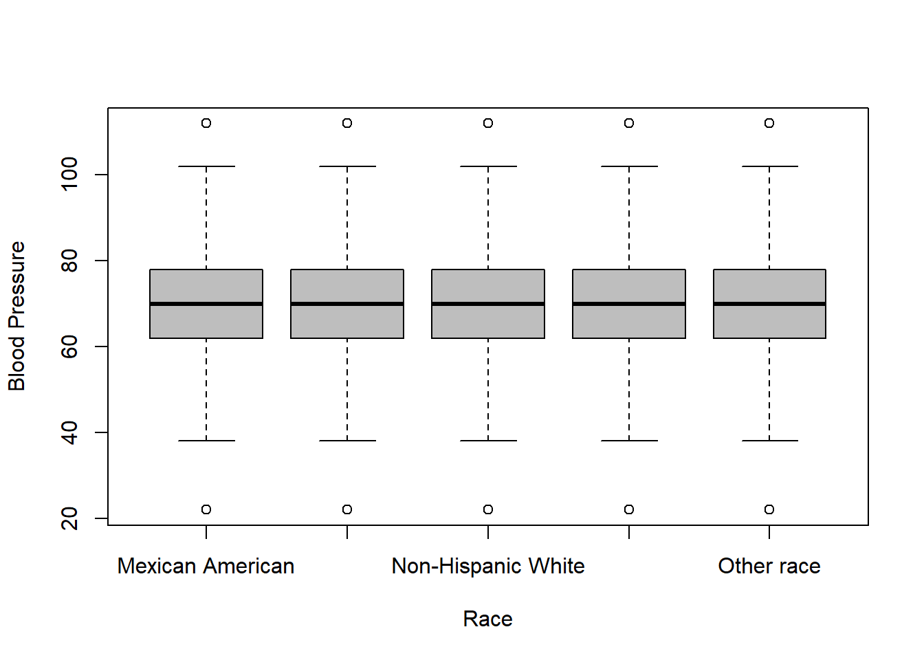
svyboxplot(blood.pressure~gender, design = analytic.design, col="grey",
           ylab="Blood Pressure",
           xlab ="Gender")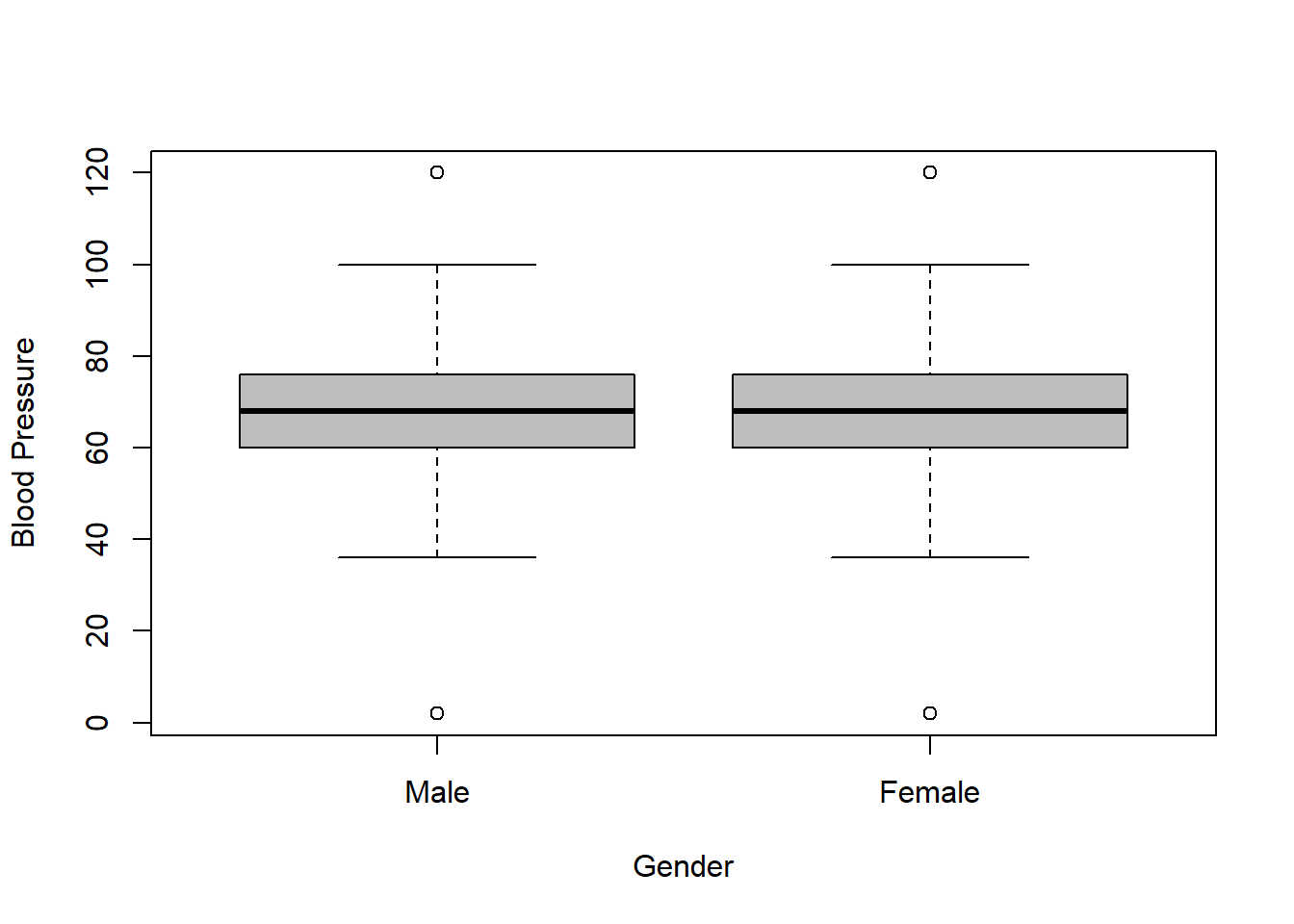
svyboxplot(blood.pressure~marital, design = analytic.design, col="grey",
           ylab="Blood Pressure",
           xlab ="Marital Status")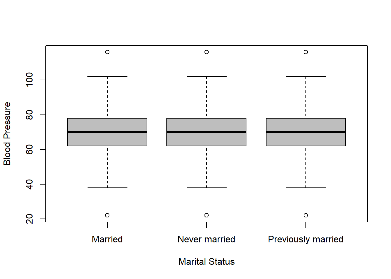
Bivariate Regression
New regression models are constructed using the survey design object to understand how each demographic variable impacts blood pressure while taking survey features into consideration.
require(survey)
summary(fit1r <- svyglm(blood.pressure ~ race, design=analytic.design))
#>
#> Call:
#> svyglm(formula = blood.pressure ~ race, design = analytic.design)
#>
#> Survey design:
#> svydesign(strata = ~SDMVSTRA, id = ~SDMVPSU, weights = ~WTMEC2YR,
#>     data = analytic.data, nest = TRUE)
#>
#> Coefficients:
#>                        Estimate Std. Error t value Pr(>|t|)
#> (Intercept)             66.6150     0.2756 241.671  < 2e-16 ***
#> raceNon-Hispanic Black   2.0491     0.6144   3.335 0.006650 **
#> raceNon-Hispanic White   1.9182     0.4269   4.493 0.000912 ***
#> raceOther Hispanic       0.2021     0.7825   0.258 0.800928
#> raceOther race           2.6091     0.3998   6.527 4.27e-05 ***
#> ---
#> Signif. codes:  0 '***' 0.001 '**' 0.01 '*' 0.05 '.' 0.1 ' ' 1
#>
#> (Dispersion parameter for gaussian family taken to be 179.8689)
#>
#> Number of Fisher Scoring iterations: 2summary(fit1a <- svyglm(blood.pressure ~ age.centred, design=analytic.design))
#>
#> Call:
#> svyglm(formula = blood.pressure ~ age.centred, design = analytic.design)
#>
#> Survey design:
#> svydesign(strata = ~SDMVSTRA, id = ~SDMVPSU, weights = ~WTMEC2YR,
#> data = analytic.data, nest = TRUE)
#>
#> Coefficients:
#> Estimate Std. Error t value Pr(>|t|)
#> (Intercept) 69.25489 0.47091 147.07 < 2e-16 ***
#> age.centred 0.15142 0.01503 10.08 8.5e-08 ***
#> ---
#> Signif. codes: 0 '***' 0.001 '**' 0.01 '*' 0.05 '.' 0.1 ' ' 1
#>
#> (Dispersion parameter for gaussian family taken to be 169.12)
#>
#> Number of Fisher Scoring iterations: 2summary(fit1g <- svyglm(blood.pressure ~ gender, design=analytic.design))
#>
#> Call:
#> svyglm(formula = blood.pressure ~ gender, design = analytic.design)
#>
#> Survey design:
#> svydesign(strata = ~SDMVSTRA, id = ~SDMVPSU, weights = ~WTMEC2YR,
#> data = analytic.data, nest = TRUE)
#>
#> Coefficients:
#> Estimate Std. Error t value Pr(>|t|)
#> (Intercept) 69.2898 0.4552 152.208 < 2e-16 ***
#> genderFemale -1.9096 0.4233 -4.511 0.000488 ***
#> ---
#> Signif. codes: 0 '***' 0.001 '**' 0.01 '*' 0.05 '.' 0.1 ' ' 1
#>
#> (Dispersion parameter for gaussian family taken to be 179.4491)
#>
#> Number of Fisher Scoring iterations: 2summary(fit1m <- svyglm(blood.pressure ~ marital, design=analytic.design))
#>
#> Call:
#> svyglm(formula = blood.pressure ~ marital, design = analytic.design)
#>
#> Survey design:
#> svydesign(strata = ~SDMVSTRA, id = ~SDMVPSU, weights = ~WTMEC2YR,
#> data = analytic.data, nest = TRUE)
#>
#> Coefficients:
#> Estimate Std. Error t value Pr(>|t|)
#> (Intercept) 70.8262 0.4978 142.265 <2e-16 ***
#> maritalNever married -1.1963 0.5482 -2.182 0.0481 *
#> maritalPreviously married -0.5038 0.4258 -1.183 0.2579
#> ---
#> Signif. codes: 0 '***' 0.001 '**' 0.01 '*' 0.05 '.' 0.1 ' ' 1
#>
#> (Dispersion parameter for gaussian family taken to be 175.0038)
#>
#> Number of Fisher Scoring iterations: 2Multivariate Regression
A final, more complex model is fitted, which includes multiple demographic variables and also considers the survey design.
analytic.design2 <- svydesign(strata=~SDMVSTRA, id=~SDMVPSU, weights=~WTMEC2YR, data=analytic.data, nest=TRUE)
summary(fit1 <- svyglm(blood.pressure ~ race + age.centred + gender + marital, design=analytic.design2))
#>
#> Call:
#> svyglm(formula = blood.pressure ~ race + age.centred + gender +
#>     marital, design = analytic.design2)
#>
#> Survey design:
#> svydesign(strata = ~SDMVSTRA, id = ~SDMVPSU, weights = ~WTMEC2YR,
#>     data = analytic.data, nest = TRUE)
#>
#> Coefficients:
#>                           Estimate Std. Error t value Pr(>|t|)
#> (Intercept)               71.14686    0.37976 187.348 3.26e-14 ***
#> raceNon-Hispanic Black     2.30248    0.84786   2.716 0.029953 *
#> raceNon-Hispanic White     1.08919    0.35921   3.032 0.019055 *
#> raceOther Hispanic         0.07339    1.20016   0.061 0.952947
#> raceOther race             2.11590    0.45579   4.642 0.002363 **
#> age.centred               -0.02223    0.01566  -1.419 0.198767
#> genderFemale              -2.91901    0.43979  -6.637 0.000294 ***
#> maritalNever married      -1.74002    0.48086  -3.619 0.008526 **
#> maritalPreviously married  0.22443    0.45139   0.497 0.634278
#> ---
#> Signif. codes:  0 '***' 0.001 '**' 0.01 '*' 0.05 '.' 0.1 ' ' 1
#>
#> (Dispersion parameter for gaussian family taken to be 171.5455)
#>
#> Number of Fisher Scoring iterations: 2
A note about Predictive models
In statistical analyses involving survey data, it’s crucial to account for the survey’s design features. These features can include sampling weights, stratification, and clustering, among others. Ignoring these could lead to biased estimates and incorrect conclusions. Considering such survey design features make the analysis more robust and reliable in terms of inference.
However, when the goal shifts from inference to prediction, additional challenges come into play. Specifically, the model may perform well on the data used to fit it (the “training” data) but not generalize well to new, unseen data. This discrepancy between training performance and generalization to new data is often referred to as “overfitting,” and the optimism of the model refers to the extent to which it overestimates its predictive performance on new data based on its performance on the training data.
Optimism-correction techniques are methodologies designed to address this issue. They allow you to evaluate how well your model is likely to perform on new data, not just the data you used to build it. Methods for optimism correction often involve techniques like cross-validation, bootstrapping, or specialized types of model validation that help in estimating the ‘true’ predictive performance of the model. Some of these techniques were discussed in the predictive modelling chapter.
Video content (optional)
For those who prefer a video walkthrough, feel free to watch the video below, which offers a description of an earlier version of the above content.