Justification
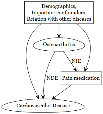
We must show enough justification to do a mediation analysis. A causal diagram would be the first step to conceptualize the mediation analysis problem hypothetically. Then, we can empirically verify where doing the mediation analysis makes sense in that particular context.
Pre-processing
Load saved data
Prepared the data
Notation
- Outcome (\(Y\)): Cardiovascular disease (CVD)
- Exposure (\(A\)): Osteoarthritis (OA)
- Mediator (\(M\)): Pain medication
- Adjustment covariates (\(C\))
Hypothesis
- For total effect (TE): Is OA (\(A\)) associated with CVD (\(Y\))?

- For mediation analysis: Does pain-medication (\(M\)) play a mediating role in the causal pathway between OA (\(A\)) and CVD (\(Y\))? Here, we will decompose total effect (TE) to a natural direct effect (NDE) and a natural indirect effect (NIE).
Adjustment variables (\(C\)):
- Demographics
- age
- sex
- income
- race
- education status
- Important confounders
- BMI
- physical activity
- smoking status
- fruit and vegetable consumption
- Relation with other diseases
- hypertension
- COPD
- diabetes
Analysis/empirical exploration
Total effect
Outcome model (weighted) is
\(logit [P(Y_{a}=1 | C = c)] = \theta_0 + \theta_1 a + \theta_3 c\)
(The subscript \(\theta_2\) is intentionally skipped here; it is reserved for the counterfactual exposure term \(a^*\) that appears later in the mediation decomposition, so the notation lines up with the Step-4 outcome model.)
Setting Design
require(survey)
summary(analytic.miss$weight)
#>    Min. 1st Qu.  Median    Mean 3rd Qu.    Max.
#>    0.39   21.76   42.21   66.70   81.07 2384.98

# Survey design
w.design0 <- svydesign(id=~1, weights=~weight, data=analytic.miss)
summary(weights(w.design0))
#>    Min. 1st Qu.  Median    Mean 3rd Qu.    Max.
#>    0.39   21.76   42.21   66.70   81.07 2384.98
sd(weights(w.design0))
#> [1] 80.34263

# Subset the design
w.design <- subset(w.design0, miss == 0)
summary(weights(w.design))
#>     Min.  1st Qu.   Median     Mean  3rd Qu.     Max.
#>    2.053   28.480   53.218   82.472  102.860 1295.970
sd(weights(w.design))
#> [1] 91.98946
# Model
TE <- svyglm(outcome ~ exposure + age + sex + income + race + bmi + edu + phyact +
smoke + fruit + diab, design = w.design, family = quasibinomial("logit"))
# painmed is mediator; not included here.
TE.save <- exp(c(summary(TE)$coef["exposure",1],
confint(TE)["exposure",]))
TE.save
#> 2.5 % 97.5 %
#> 1.537005 1.230735 1.919489Exposure to OA has a detrimental effect on CVD risk (significant!).
Effect on the mediators
fit.m = svyglm(mediator ~ exposure + age + sex + income + race + bmi + edu +
                 phyact + smoke + fruit + diab, design = w.design,
               family = binomial("logit"))
#> Warning in eval(family$initialize): non-integer #successes in a binomial glm!
med.save <- exp(c(summary(fit.m)$coef["exposure",1], confint(fit.m)["exposure",]))
med.save
#>             2.5 %   97.5 %
#> 2.428463 2.059265 2.863853
Exposure to OA has a substantial effect on the mediator (Pain medication) as well (significant!). Hence, it would be interesting to explore a mediation analysis to assess the mediating role.
Save data
Video content (optional)
For those who prefer a video walkthrough, feel free to watch the video below, which offers a description of an earlier version of the above content.