Imputation in NHANES

This tutorial provides a comprehensive guide on handling and analyzing complex survey data with missing values. In analyzing complex survey data, a distinct approach is required compared to handling regular datasets. Specifically, the intricacies of survey design necessitate the consideration of primary sampling units/cluster, sampling weights, and stratification factors. These elements ensure that the analysis accurately reflects the survey’s design and the underlying population structure. Recognizing and incorporating these factors is crucial for obtaining valid and representative insights from the data. As we delve into this tutorial, we’ll explore how to effectively integrate these components into our missing data analysis process.

Complex Survey data

In the initial chunk, we load all the necessary libraries that will be used throughout the tutorial. These libraries provide functions and tools for data exploration, visualization, imputation, and analysis.

# Load required packages
library(mice)
library(DataExplorer)
library(VIM)
library(jtools)
library(survey)
library(mitools)

Next, we load a dataset that contains survey data with some missing values. We then select specific columns or variables from this dataset that we are interested in analyzing. To understand the extent and pattern of missingness in our data, we visualize it and display the missing data pattern.

load("Data/missingdata/NHANES17.RData")

Vars <- c("ID", "weight", "psu", "strata", 
          "gender", "born", "race", 
          "bmi", "cholesterol", "diabetes")
analyticx <- analytic.with.miss[,Vars]
plot_missing(analyticx)

md.pattern(analyticx)

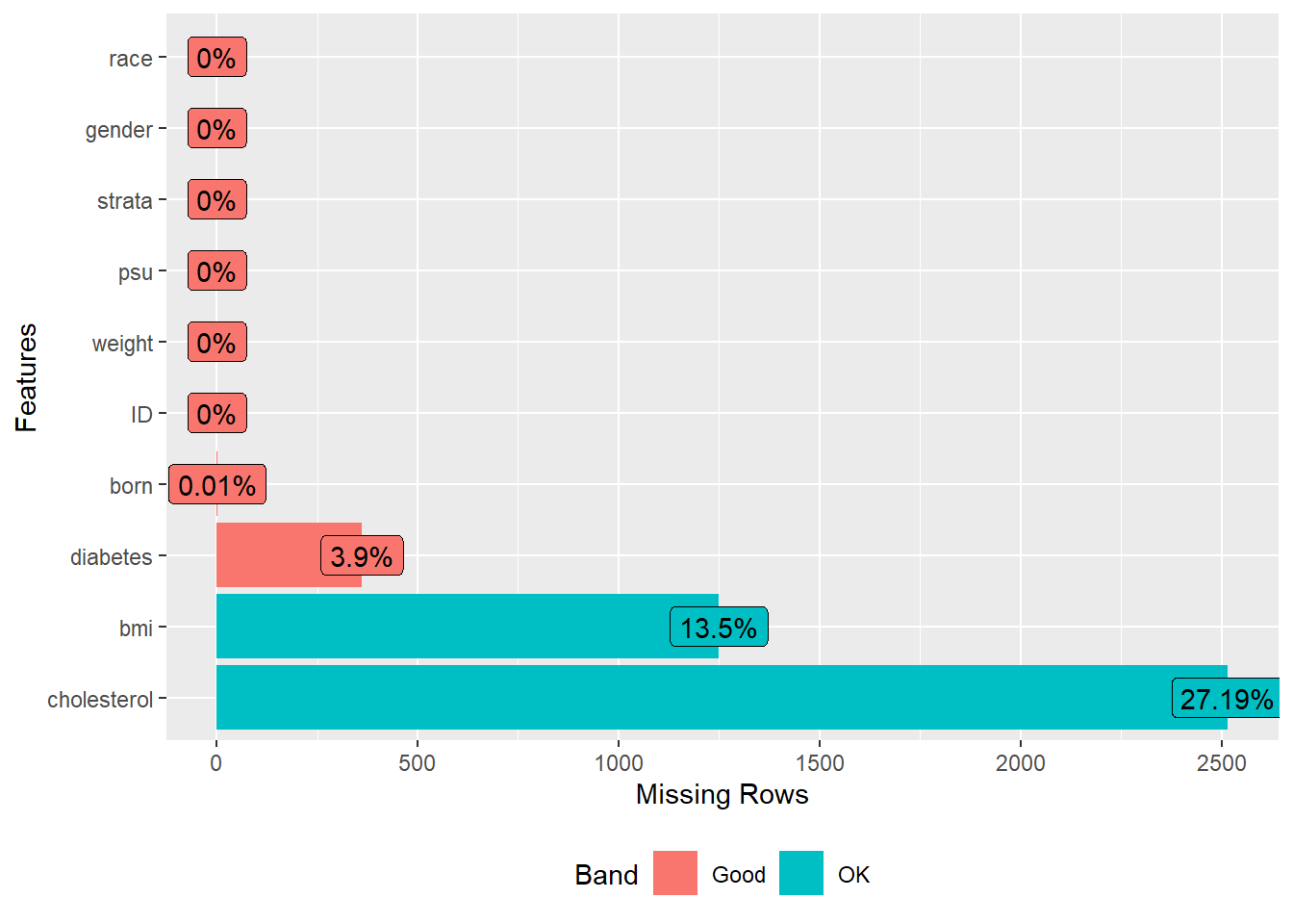
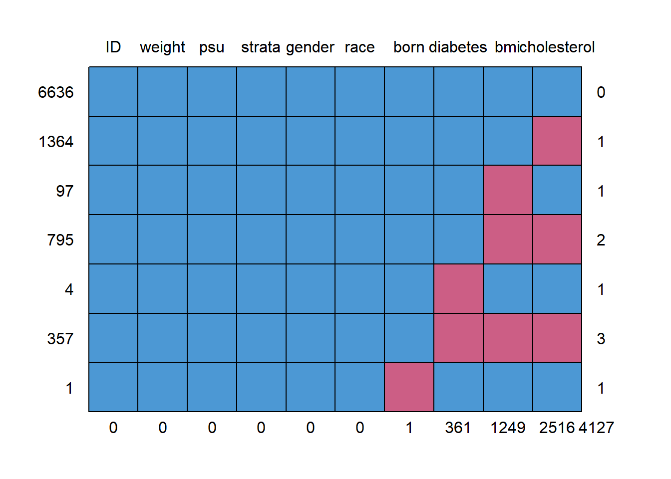
#>      ID weight psu strata gender race born diabetes  bmi cholesterol     
#> 6636  1      1   1      1      1    1    1        1    1           1    0
#> 1364  1      1   1      1      1    1    1        1    1           0    1
#> 97    1      1   1      1      1    1    1        1    0           1    1
#> 795   1      1   1      1      1    1    1        1    0           0    2
#> 4     1      1   1      1      1    1    1        0    1           1    1
#> 357   1      1   1      1      1    1    1        0    0           0    3
#> 1     1      1   1      1      1    1    0        1    1           1    1
#>       0      0   0      0      0    0    1      361 1249        2516 4127

Imputing

In the following chunk, we address the missing data by performing multiple imputations. This means that instead of filling in each missing value with a single estimate, we create multiple versions (datasets) where each missing value is filled in differently based on a specified algorithm. This helps in capturing the uncertainty around the missing values. The chunk sets up the parameters for multiple imputations, ensuring reproducibility and efficiency, and then performs the imputations on the dataset with missing values.

# imputation <- mice(analyticx, m=5, maxit=5, seed = 504007)
set.seed(504)
imputation <- parlmice(analyticx, m=5, maxit=5, cluster.seed=504007)
#> Warning: 'parlmice' is deprecated.
#> Use 'futuremice' instead.
#> See help("Deprecated")

Data Input: The primary input for the imputation function is the dataset with missing values. This dataset is what we aim to impute.
Number of Imputations: The option m=5 indicates that we want to create 5 different imputed datasets. Each of these datasets will have the missing values filled in slightly differently, based on the underlying imputation algorithm and the randomness introduced.
Maximum Iterations: The imputation process is iterative, meaning it refines its estimates over several rounds. The option maxit=5 specifies that the algorithm should run for a maximum of 5 iterations. This helps in achieving more accurate imputations, especially when the missing data mechanism is complex.
Setting Seed: In computational processes that involve randomness, it’s often useful to set a “seed” value. This ensures that the random processes are reproducible. If you run the imputation multiple times with the same seed, you’ll get the same results each time. Two seed values are set in the chunk: one using the general set.seed() function and another specifically for the imputation function as cluster.seed.
Parallel Processing: The function parlmice used for imputation indicates that the imputations are done in parallel. This means that instead of imputing one dataset after the other, the function tries to impute multiple datasets simultaneously (if the computational resources allow). This can speed up the process, especially when dealing with large datasets or when creating many imputed datasets.

Create new variable

After imputation, we might want to create new variables or modify existing ones to better suit our analysis. Here, we transform one of the variables into a binary category based on a threshold. The choice of thresholds should be based on the data (i.e. median, quintiles, etc.) or on the literature (clinically relevant). This can help in simplifying the analysis or making the results more interpretable.

impdata <- complete(imputation, action="long") #stacked data
impdata$cholesterol.bin <- ifelse(impdata$cholesterol < 200, "healthy", "unhealthy")
impdata$cholesterol.bin <- as.factor(impdata$cholesterol.bin)
dim(impdata)
#> [1] 46270    13
head(impdata)

Checking the data

After imputation, it’s crucial to ensure that the imputed data maintains the integrity and structure of the original dataset. The following chunks are designed to help you visually and programmatically inspect the imputed data.

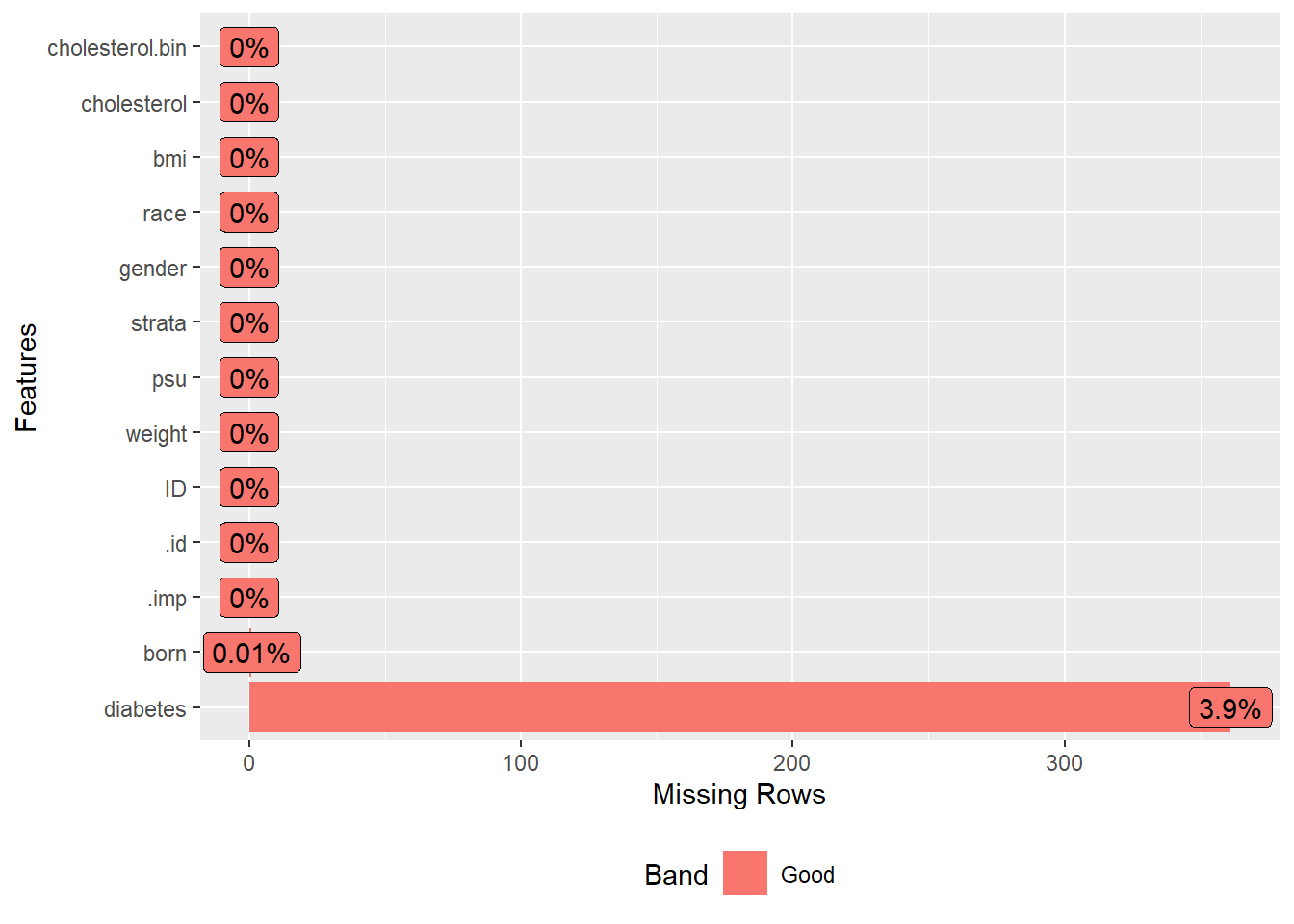
Visual Inspection of Missing Data:

In this chunk, we visually inspect the imputed datasets to see if there are any remaining missing values. We specifically look at the first two imputed datasets. Visualization tools like these can quickly show if the imputation process was successful in filling all missing values.

plot_missing(subset(impdata, subset=.imp==1))

plot_missing(subset(impdata, subset=.imp==2))

Comparing Original and Imputed Data (First Imputed Dataset):

In this chunk, we focus on the first imputed dataset. We extract this dataset and display the initial entries to get a sense of the data.
We then remove any remaining missing values (if any) and display the initial entries of this complete dataset.
Next, we compare the IDs (or unique identifiers) of the entries in the complete dataset with the original dataset to see which entries had missing values.
We then create a new variable that indicates whether an entry had missing values or not and tabulate this information.

analytic.miss1 <- subset(impdata, subset=.imp==1)
head(analytic.miss1$ID) # full data
#> [1] 93703 93704 93705 93706 93707 93708

analytic1 <- as.data.frame(na.omit(analytic.miss1))
head(analytic1$ID) # complete case
#> [1] 93703 93704 93705 93706 93707 93708

head(analytic.miss1$ID[analytic.miss1$ID %in% analytic1$ID])
#> [1] 93703 93704 93705 93706 93707 93708

analytic.miss1$miss <- 1
analytic.miss1$miss[analytic.miss1$ID %in% analytic1$ID] <- 0
table(analytic.miss1$miss)
#> 
#>    0    1 
#> 8892  362

head(analytic.miss1$ID[analytic.miss1$miss==1])
#> [1] 93710 93748 93786 93854 93865 93934
tail(analytic.miss1$ID[analytic.miss1$miss==1])
#> [1] 102840 102862 102919 102927 102928 102942

Comparing Original and Imputed Data (Second Imputed Dataset):

The this chunk is similar to the above but focuses on the second imputed dataset. We perform the same steps: extracting the dataset, removing missing values, comparing IDs, and creating a variable to indicate missingness.

analytic.miss2 <- subset(impdata, subset=.imp==2)
head(analytic.miss2$ID) # full data
#> [1] 93703 93704 93705 93706 93707 93708

analytic2 <- as.data.frame(na.omit(analytic.miss2))
head(analytic2$ID) # complete case
#> [1] 93703 93704 93705 93706 93707 93708

head(analytic.miss2$ID[analytic.miss2$ID %in% analytic2$ID])
#> [1] 93703 93704 93705 93706 93707 93708

analytic.miss2$miss <- 1
analytic.miss2$miss[analytic.miss2$ID %in% analytic2$ID] <- 0
table(analytic.miss2$miss)
#> 
#>    0    1 
#> 8892  362

head(analytic.miss1$ID[analytic.miss1$miss==1])
#> [1] 93710 93748 93786 93854 93865 93934
tail(analytic.miss1$ID[analytic.miss1$miss==1])
#> [1] 102840 102862 102919 102927 102928 102942

Aggregating Missingness Information Across All Imputed Datasets:

In the fourth chunk, we aim to consolidate the missingness information across all imputed datasets. We initialize a variable in the main dataset to indicate missingness.
We then loop through each of the imputed datasets and update the main dataset’s missingness variable based on the missingness information from each imputed dataset. This gives us a consolidated view of which entries had missing values across all imputed datasets.

impdata$miss<-1
m <- 5
for (i in 1:m){
  impdata$miss[impdata$.imp == i] <- analytic.miss2$miss
  print(table(impdata$miss[impdata$.imp == i]))
}
#> 
#>    0    1 
#> 8892  362 
#> 
#>    0    1 
#> 8892  362 
#> 
#>    0    1 
#> 8892  362 
#> 
#>    0    1 
#> 8892  362 
#> 
#>    0    1 
#> 8892  362

Combining data

Since we have multiple versions of the imputed dataset, we need a way to combine them for analysis. In the next chunks, we use a method to merge these datasets into a single list, making it easier to apply subsequent analyses on all datasets simultaneously.

library(mitools) 
allImputations <- imputationList(list(
  subset(impdata, subset=.imp==1),
  subset(impdata, subset=.imp==2),
  subset(impdata, subset=.imp==3),
  subset(impdata, subset=.imp==4), 
  subset(impdata, subset=.imp==5)))
str(allImputations)
#> List of 2
#>  $ imputations:List of 5
#>   ..$ :'data.frame': 9254 obs. of  14 variables:
#>   .. ..$ .imp           : int [1:9254] 1 1 1 1 1 1 1 1 1 1 ...
#>   .. ..$ .id            : int [1:9254] 1 2 3 4 5 6 7 8 9 10 ...
#>   .. ..$ ID             : int [1:9254] 93703 93704 93705 93706 93707 93708 93709 93710 93711 93712 ...
#>   .. ..$ weight         : num [1:9254] 8540 42567 8338 8723 7065 ...
#>   .. ..$ psu            : Factor w/ 2 levels "1","2": 2 1 2 2 1 2 1 1 2 2 ...
#>   .. ..$ strata         : Factor w/ 15 levels "134","135","136",..: 12 10 12 1 5 5 3 1 1 14 ...
#>   .. ..$ gender         : chr [1:9254] "Female" "Male" "Female" "Male" ...
#>   .. ..$ born           : chr [1:9254] "Born in 50 US states or Washingt" "Born in 50 US states or Washingt" "Born in 50 US states or Washingt" "Born in 50 US states or Washingt" ...
#>   .. ..$ race           : chr [1:9254] "Other" "White" "Black" "Other" ...
#>   .. ..$ bmi            : num [1:9254] 17.5 15.7 31.7 21.5 18.1 23.7 38.9 18.3 21.3 19.7 ...
#>   .. ..$ cholesterol    : int [1:9254] 160 186 157 148 189 209 176 162 238 182 ...
#>   .. ..$ diabetes       : chr [1:9254] "No" "No" "No" "No" ...
#>   .. ..$ cholesterol.bin: Factor w/ 2 levels "healthy","unhealthy": 1 1 1 1 1 2 1 1 2 1 ...
#>   .. ..$ miss           : num [1:9254] 0 0 0 0 0 0 0 1 0 0 ...
#>   ..$ :'data.frame': 9254 obs. of  14 variables:
#>   .. ..$ .imp           : int [1:9254] 2 2 2 2 2 2 2 2 2 2 ...
#>   .. ..$ .id            : int [1:9254] 1 2 3 4 5 6 7 8 9 10 ...
#>   .. ..$ ID             : int [1:9254] 93703 93704 93705 93706 93707 93708 93709 93710 93711 93712 ...
#>   .. ..$ weight         : num [1:9254] 8540 42567 8338 8723 7065 ...
#>   .. ..$ psu            : Factor w/ 2 levels "1","2": 2 1 2 2 1 2 1 1 2 2 ...
#>   .. ..$ strata         : Factor w/ 15 levels "134","135","136",..: 12 10 12 1 5 5 3 1 1 14 ...
#>   .. ..$ gender         : chr [1:9254] "Female" "Male" "Female" "Male" ...
#>   .. ..$ born           : chr [1:9254] "Born in 50 US states or Washingt" "Born in 50 US states or Washingt" "Born in 50 US states or Washingt" "Born in 50 US states or Washingt" ...
#>   .. ..$ race           : chr [1:9254] "Other" "White" "Black" "Other" ...
#>   .. ..$ bmi            : num [1:9254] 17.5 15.7 31.7 21.5 18.1 23.7 38.9 44.8 21.3 19.7 ...
#>   .. ..$ cholesterol    : int [1:9254] 107 153 157 148 189 209 176 195 238 182 ...
#>   .. ..$ diabetes       : chr [1:9254] "No" "No" "No" "No" ...
#>   .. ..$ cholesterol.bin: Factor w/ 2 levels "healthy","unhealthy": 1 1 1 1 1 2 1 1 2 1 ...
#>   .. ..$ miss           : num [1:9254] 0 0 0 0 0 0 0 1 0 0 ...
#>   ..$ :'data.frame': 9254 obs. of  14 variables:
#>   .. ..$ .imp           : int [1:9254] 3 3 3 3 3 3 3 3 3 3 ...
#>   .. ..$ .id            : int [1:9254] 1 2 3 4 5 6 7 8 9 10 ...
#>   .. ..$ ID             : int [1:9254] 93703 93704 93705 93706 93707 93708 93709 93710 93711 93712 ...
#>   .. ..$ weight         : num [1:9254] 8540 42567 8338 8723 7065 ...
#>   .. ..$ psu            : Factor w/ 2 levels "1","2": 2 1 2 2 1 2 1 1 2 2 ...
#>   .. ..$ strata         : Factor w/ 15 levels "134","135","136",..: 12 10 12 1 5 5 3 1 1 14 ...
#>   .. ..$ gender         : chr [1:9254] "Female" "Male" "Female" "Male" ...
#>   .. ..$ born           : chr [1:9254] "Born in 50 US states or Washingt" "Born in 50 US states or Washingt" "Born in 50 US states or Washingt" "Born in 50 US states or Washingt" ...
#>   .. ..$ race           : chr [1:9254] "Other" "White" "Black" "Other" ...
#>   .. ..$ bmi            : num [1:9254] 17.5 15.7 31.7 21.5 18.1 23.7 38.9 13.6 21.3 19.7 ...
#>   .. ..$ cholesterol    : int [1:9254] 153 110 157 148 189 209 176 141 238 182 ...
#>   .. ..$ diabetes       : chr [1:9254] "No" "No" "No" "No" ...
#>   .. ..$ cholesterol.bin: Factor w/ 2 levels "healthy","unhealthy": 1 1 1 1 1 2 1 1 2 1 ...
#>   .. ..$ miss           : num [1:9254] 0 0 0 0 0 0 0 1 0 0 ...
#>   ..$ :'data.frame': 9254 obs. of  14 variables:
#>   .. ..$ .imp           : int [1:9254] 4 4 4 4 4 4 4 4 4 4 ...
#>   .. ..$ .id            : int [1:9254] 1 2 3 4 5 6 7 8 9 10 ...
#>   .. ..$ ID             : int [1:9254] 93703 93704 93705 93706 93707 93708 93709 93710 93711 93712 ...
#>   .. ..$ weight         : num [1:9254] 8540 42567 8338 8723 7065 ...
#>   .. ..$ psu            : Factor w/ 2 levels "1","2": 2 1 2 2 1 2 1 1 2 2 ...
#>   .. ..$ strata         : Factor w/ 15 levels "134","135","136",..: 12 10 12 1 5 5 3 1 1 14 ...
#>   .. ..$ gender         : chr [1:9254] "Female" "Male" "Female" "Male" ...
#>   .. ..$ born           : chr [1:9254] "Born in 50 US states or Washingt" "Born in 50 US states or Washingt" "Born in 50 US states or Washingt" "Born in 50 US states or Washingt" ...
#>   .. ..$ race           : chr [1:9254] "Other" "White" "Black" "Other" ...
#>   .. ..$ bmi            : num [1:9254] 17.5 15.7 31.7 21.5 18.1 23.7 38.9 19.2 21.3 19.7 ...
#>   .. ..$ cholesterol    : int [1:9254] 160 159 157 148 189 209 176 196 238 182 ...
#>   .. ..$ diabetes       : chr [1:9254] "No" "No" "No" "No" ...
#>   .. ..$ cholesterol.bin: Factor w/ 2 levels "healthy","unhealthy": 1 1 1 1 1 2 1 1 2 1 ...
#>   .. ..$ miss           : num [1:9254] 0 0 0 0 0 0 0 1 0 0 ...
#>   ..$ :'data.frame': 9254 obs. of  14 variables:
#>   .. ..$ .imp           : int [1:9254] 5 5 5 5 5 5 5 5 5 5 ...
#>   .. ..$ .id            : int [1:9254] 1 2 3 4 5 6 7 8 9 10 ...
#>   .. ..$ ID             : int [1:9254] 93703 93704 93705 93706 93707 93708 93709 93710 93711 93712 ...
#>   .. ..$ weight         : num [1:9254] 8540 42567 8338 8723 7065 ...
#>   .. ..$ psu            : Factor w/ 2 levels "1","2": 2 1 2 2 1 2 1 1 2 2 ...
#>   .. ..$ strata         : Factor w/ 15 levels "134","135","136",..: 12 10 12 1 5 5 3 1 1 14 ...
#>   .. ..$ gender         : chr [1:9254] "Female" "Male" "Female" "Male" ...
#>   .. ..$ born           : chr [1:9254] "Born in 50 US states or Washingt" "Born in 50 US states or Washingt" "Born in 50 US states or Washingt" "Born in 50 US states or Washingt" ...
#>   .. ..$ race           : chr [1:9254] "Other" "White" "Black" "Other" ...
#>   .. ..$ bmi            : num [1:9254] 17.5 15.7 31.7 21.5 18.1 23.7 38.9 26 21.3 19.7 ...
#>   .. ..$ cholesterol    : int [1:9254] 132 198 157 148 189 209 176 255 238 182 ...
#>   .. ..$ diabetes       : chr [1:9254] "No" "No" "No" "No" ...
#>   .. ..$ cholesterol.bin: Factor w/ 2 levels "healthy","unhealthy": 1 1 1 1 1 2 1 2 2 1 ...
#>   .. ..$ miss           : num [1:9254] 0 0 0 0 0 0 0 1 0 0 ...
#>  $ call       : language imputationList(list(subset(impdata, subset = .imp == 1), subset(impdata,      subset = .imp == 2), subset(impdata| __truncated__ ...
#>  - attr(*, "class")= chr "imputationList"

Combining data efficiently

m <- 5
set.seed(123)
allImputations <-  imputationList(lapply(1:m, 
                                         function(n)  
                                           subset(impdata, subset=.imp==n)))
                                           #mice::complete(imputation, action = n)))
summary(allImputations)
#>             Length Class  Mode
#> imputations 5      -none- list
#> call        2      -none- call
str(allImputations)
#> List of 2
#>  $ imputations:List of 5
#>   ..$ :'data.frame': 9254 obs. of  14 variables:
#>   .. ..$ .imp           : int [1:9254] 1 1 1 1 1 1 1 1 1 1 ...
#>   .. ..$ .id            : int [1:9254] 1 2 3 4 5 6 7 8 9 10 ...
#>   .. ..$ ID             : int [1:9254] 93703 93704 93705 93706 93707 93708 93709 93710 93711 93712 ...
#>   .. ..$ weight         : num [1:9254] 8540 42567 8338 8723 7065 ...
#>   .. ..$ psu            : Factor w/ 2 levels "1","2": 2 1 2 2 1 2 1 1 2 2 ...
#>   .. ..$ strata         : Factor w/ 15 levels "134","135","136",..: 12 10 12 1 5 5 3 1 1 14 ...
#>   .. ..$ gender         : chr [1:9254] "Female" "Male" "Female" "Male" ...
#>   .. ..$ born           : chr [1:9254] "Born in 50 US states or Washingt" "Born in 50 US states or Washingt" "Born in 50 US states or Washingt" "Born in 50 US states or Washingt" ...
#>   .. ..$ race           : chr [1:9254] "Other" "White" "Black" "Other" ...
#>   .. ..$ bmi            : num [1:9254] 17.5 15.7 31.7 21.5 18.1 23.7 38.9 18.3 21.3 19.7 ...
#>   .. ..$ cholesterol    : int [1:9254] 160 186 157 148 189 209 176 162 238 182 ...
#>   .. ..$ diabetes       : chr [1:9254] "No" "No" "No" "No" ...
#>   .. ..$ cholesterol.bin: Factor w/ 2 levels "healthy","unhealthy": 1 1 1 1 1 2 1 1 2 1 ...
#>   .. ..$ miss           : num [1:9254] 0 0 0 0 0 0 0 1 0 0 ...
#>   ..$ :'data.frame': 9254 obs. of  14 variables:
#>   .. ..$ .imp           : int [1:9254] 2 2 2 2 2 2 2 2 2 2 ...
#>   .. ..$ .id            : int [1:9254] 1 2 3 4 5 6 7 8 9 10 ...
#>   .. ..$ ID             : int [1:9254] 93703 93704 93705 93706 93707 93708 93709 93710 93711 93712 ...
#>   .. ..$ weight         : num [1:9254] 8540 42567 8338 8723 7065 ...
#>   .. ..$ psu            : Factor w/ 2 levels "1","2": 2 1 2 2 1 2 1 1 2 2 ...
#>   .. ..$ strata         : Factor w/ 15 levels "134","135","136",..: 12 10 12 1 5 5 3 1 1 14 ...
#>   .. ..$ gender         : chr [1:9254] "Female" "Male" "Female" "Male" ...
#>   .. ..$ born           : chr [1:9254] "Born in 50 US states or Washingt" "Born in 50 US states or Washingt" "Born in 50 US states or Washingt" "Born in 50 US states or Washingt" ...
#>   .. ..$ race           : chr [1:9254] "Other" "White" "Black" "Other" ...
#>   .. ..$ bmi            : num [1:9254] 17.5 15.7 31.7 21.5 18.1 23.7 38.9 44.8 21.3 19.7 ...
#>   .. ..$ cholesterol    : int [1:9254] 107 153 157 148 189 209 176 195 238 182 ...
#>   .. ..$ diabetes       : chr [1:9254] "No" "No" "No" "No" ...
#>   .. ..$ cholesterol.bin: Factor w/ 2 levels "healthy","unhealthy": 1 1 1 1 1 2 1 1 2 1 ...
#>   .. ..$ miss           : num [1:9254] 0 0 0 0 0 0 0 1 0 0 ...
#>   ..$ :'data.frame': 9254 obs. of  14 variables:
#>   .. ..$ .imp           : int [1:9254] 3 3 3 3 3 3 3 3 3 3 ...
#>   .. ..$ .id            : int [1:9254] 1 2 3 4 5 6 7 8 9 10 ...
#>   .. ..$ ID             : int [1:9254] 93703 93704 93705 93706 93707 93708 93709 93710 93711 93712 ...
#>   .. ..$ weight         : num [1:9254] 8540 42567 8338 8723 7065 ...
#>   .. ..$ psu            : Factor w/ 2 levels "1","2": 2 1 2 2 1 2 1 1 2 2 ...
#>   .. ..$ strata         : Factor w/ 15 levels "134","135","136",..: 12 10 12 1 5 5 3 1 1 14 ...
#>   .. ..$ gender         : chr [1:9254] "Female" "Male" "Female" "Male" ...
#>   .. ..$ born           : chr [1:9254] "Born in 50 US states or Washingt" "Born in 50 US states or Washingt" "Born in 50 US states or Washingt" "Born in 50 US states or Washingt" ...
#>   .. ..$ race           : chr [1:9254] "Other" "White" "Black" "Other" ...
#>   .. ..$ bmi            : num [1:9254] 17.5 15.7 31.7 21.5 18.1 23.7 38.9 13.6 21.3 19.7 ...
#>   .. ..$ cholesterol    : int [1:9254] 153 110 157 148 189 209 176 141 238 182 ...
#>   .. ..$ diabetes       : chr [1:9254] "No" "No" "No" "No" ...
#>   .. ..$ cholesterol.bin: Factor w/ 2 levels "healthy","unhealthy": 1 1 1 1 1 2 1 1 2 1 ...
#>   .. ..$ miss           : num [1:9254] 0 0 0 0 0 0 0 1 0 0 ...
#>   ..$ :'data.frame': 9254 obs. of  14 variables:
#>   .. ..$ .imp           : int [1:9254] 4 4 4 4 4 4 4 4 4 4 ...
#>   .. ..$ .id            : int [1:9254] 1 2 3 4 5 6 7 8 9 10 ...
#>   .. ..$ ID             : int [1:9254] 93703 93704 93705 93706 93707 93708 93709 93710 93711 93712 ...
#>   .. ..$ weight         : num [1:9254] 8540 42567 8338 8723 7065 ...
#>   .. ..$ psu            : Factor w/ 2 levels "1","2": 2 1 2 2 1 2 1 1 2 2 ...
#>   .. ..$ strata         : Factor w/ 15 levels "134","135","136",..: 12 10 12 1 5 5 3 1 1 14 ...
#>   .. ..$ gender         : chr [1:9254] "Female" "Male" "Female" "Male" ...
#>   .. ..$ born           : chr [1:9254] "Born in 50 US states or Washingt" "Born in 50 US states or Washingt" "Born in 50 US states or Washingt" "Born in 50 US states or Washingt" ...
#>   .. ..$ race           : chr [1:9254] "Other" "White" "Black" "Other" ...
#>   .. ..$ bmi            : num [1:9254] 17.5 15.7 31.7 21.5 18.1 23.7 38.9 19.2 21.3 19.7 ...
#>   .. ..$ cholesterol    : int [1:9254] 160 159 157 148 189 209 176 196 238 182 ...
#>   .. ..$ diabetes       : chr [1:9254] "No" "No" "No" "No" ...
#>   .. ..$ cholesterol.bin: Factor w/ 2 levels "healthy","unhealthy": 1 1 1 1 1 2 1 1 2 1 ...
#>   .. ..$ miss           : num [1:9254] 0 0 0 0 0 0 0 1 0 0 ...
#>   ..$ :'data.frame': 9254 obs. of  14 variables:
#>   .. ..$ .imp           : int [1:9254] 5 5 5 5 5 5 5 5 5 5 ...
#>   .. ..$ .id            : int [1:9254] 1 2 3 4 5 6 7 8 9 10 ...
#>   .. ..$ ID             : int [1:9254] 93703 93704 93705 93706 93707 93708 93709 93710 93711 93712 ...
#>   .. ..$ weight         : num [1:9254] 8540 42567 8338 8723 7065 ...
#>   .. ..$ psu            : Factor w/ 2 levels "1","2": 2 1 2 2 1 2 1 1 2 2 ...
#>   .. ..$ strata         : Factor w/ 15 levels "134","135","136",..: 12 10 12 1 5 5 3 1 1 14 ...
#>   .. ..$ gender         : chr [1:9254] "Female" "Male" "Female" "Male" ...
#>   .. ..$ born           : chr [1:9254] "Born in 50 US states or Washingt" "Born in 50 US states or Washingt" "Born in 50 US states or Washingt" "Born in 50 US states or Washingt" ...
#>   .. ..$ race           : chr [1:9254] "Other" "White" "Black" "Other" ...
#>   .. ..$ bmi            : num [1:9254] 17.5 15.7 31.7 21.5 18.1 23.7 38.9 26 21.3 19.7 ...
#>   .. ..$ cholesterol    : int [1:9254] 132 198 157 148 189 209 176 255 238 182 ...
#>   .. ..$ diabetes       : chr [1:9254] "No" "No" "No" "No" ...
#>   .. ..$ cholesterol.bin: Factor w/ 2 levels "healthy","unhealthy": 1 1 1 1 1 2 1 2 2 1 ...
#>   .. ..$ miss           : num [1:9254] 0 0 0 0 0 0 0 1 0 0 ...
#>  $ call       : language imputationList(lapply(1:m, function(n) subset(impdata, subset = .imp ==      n)))
#>  - attr(*, "class")= chr "imputationList"

Logistic regression

With our imputed datasets ready, we proceed to fit a statistical model. Here, we use logistic regression as an example. We fit the model to each imputed dataset separately and then extract relevant statistics like odds ratios and confidence intervals.

require(jtools)
require(survey)
data.list <- vector("list", m)
model.formula <- as.formula("I(cholesterol.bin=='healthy')~diabetes+gender+born+race+bmi")

summary(allImputations$imputations[[1]]$weight)
#>    Min. 1st Qu.  Median    Mean 3rd Qu.    Max. 
#>       0   12347   21060   34671   37562  419763
sum(allImputations$imputations[[1]]$weight==0)
#> [1] 550
w.design0 <- svydesign(ids=~psu, weights=~weight, strata=~strata,
                           data = allImputations, nest = TRUE)
w.design <- subset(w.design0, miss == 0)
fits <- with(w.design, svyglm(model.formula, family=quasibinomial))
#> Warning in summary.glm(g): observations with zero weight not used for
#> calculating dispersion
#> Warning in summary.glm(glm.object): observations with zero weight not used for
#> calculating dispersion
#> Warning in summary.glm(g): observations with zero weight not used for
#> calculating dispersion
#> Warning in summary.glm(glm.object): observations with zero weight not used for
#> calculating dispersion
#> Warning in summary.glm(g): observations with zero weight not used for
#> calculating dispersion
#> Warning in summary.glm(glm.object): observations with zero weight not used for
#> calculating dispersion
#> Warning in summary.glm(g): observations with zero weight not used for
#> calculating dispersion
#> Warning in summary.glm(glm.object): observations with zero weight not used for
#> calculating dispersion
#> Warning in summary.glm(g): observations with zero weight not used for
#> calculating dispersion
#> Warning in summary.glm(glm.object): observations with zero weight not used for
#> calculating dispersion
# Estimate from first data
exp(coef(fits[[1]]))[2]
#> diabetesYes 
#>    1.409246
exp(confint(fits[[1]]))[2,]
#>    2.5 %   97.5 % 
#> 1.129997 1.757503
# Estimate from second data
exp(coef(fits[[2]]))[2]
#> diabetesYes 
#>    1.437951
exp(confint(fits[[2]]))[2,]
#>    2.5 %   97.5 % 
#> 1.171160 1.765518

Pooled / averaged estimates

After analyzing each imputed dataset separately, we need to combine the results to get a single set of estimates. This is done using a method that pools the results, taking into account the variability between the different imputed datasets.

pooled.estimates <- MIcombine(fits)
sum.pooled <- summary(pooled.estimates)
#> Multiple imputation results:
#>       with(w.design, svyglm(model.formula, family = quasibinomial))
#>       MIcombine.default(fits)
#>                   results          se        (lower       upper) missInfo
#> (Intercept)    2.13514754 0.236310332   1.667691110   2.60260397     19 %
#> diabetesYes    0.35209050 0.089197557   0.177261457   0.52691955      1 %
#> genderMale     0.17677460 0.088502097   0.003168621   0.35038058      5 %
#> bornOthers    -0.59642404 0.096782869  -0.786797572  -0.40605051     11 %
#> bornRefused  -12.33262819 0.708505945 -13.721274703 -10.94398169      0 %
#> raceHispanic   0.13913500 0.142910787  -0.141238429   0.41950842      6 %
#> raceOther     -0.17347602 0.105412185  -0.380201753   0.03324971      5 %
#> raceWhite     -0.35812104 0.134733737  -0.622240268  -0.09400181      2 %
#> bmi           -0.04011243 0.006523474  -0.053037557  -0.02718730     20 %
exp(sum.pooled[,1])
#> [1] 8.458294e+00 1.422037e+00 1.193362e+00 5.507777e-01 4.405626e-06
#> [6] 1.149279e+00 8.407373e-01 6.989885e-01 9.606814e-01
OR <- round(exp(pooled.estimates$coefficients),2) 
OR <- as.data.frame(OR)
CI <- round(exp(confint(pooled.estimates)),2)
sig <- (CI[,1] < 1 & CI[,2] > 1)
sig <- ifelse(sig==FALSE, "*", "")
OR <- cbind(OR,CI,sig)
OR

Step-by-step example

This segment offers a hands-on approach to understanding the imputation process. Here’s a breakdown:

Fitting Models to Individual Imputed Datasets:
- A list is initialized to store the results of models fitted to each imputed dataset.
- For every dataset, the specific imputed data is extracted.
- A survey design is established, considering factors like primary sampling units, stratification, and weights. This ensures the analysis aligns with the survey’s design.
- This design is then refined to only consider complete data entries.
- A logistic regression model is then applied to this refined data.
- The results of this modeling are stored and displayed for review.
Pooling Results from All Models:
- After individual analysis, the next step is to combine or ‘pool’ these results.
- A special function is used to merge the results from all the models. This function accounts for variations between datasets and offers a combined estimate.
- A summary of this combined data is then displayed, offering insights like coefficients, standard errors, and more. Another version of this summary, focusing on log-effects, is also presented for deeper insights.

fits2 <- vector("list", m)
for (i in 1:m) {
  analytic.i <- allImputations$imputations[[i]]
  w.design0.i <- svydesign(id=~psu, strata=~strata, weights=~weight,
                        data=analytic.i, nest = TRUE)
  w.design.i <- subset(w.design0.i, miss == 0)
  fit <- svyglm(model.formula, design=w.design.i, 
                family = quasibinomial("logit"))
  print(summ(fit))
  fits2[[i]] <- fit
}
#> Warning in summary.glm(g): observations with zero weight not used for
#> calculating dispersion
#> Warning in summary.glm(glm.object): observations with zero weight not used for
#> calculating dispersion
#> MODEL INFO:
#> Observations: 8892
#> Dependent Variable: I(cholesterol.bin == "healthy")
#> Type: Analysis of complex survey design 
#>  Family: quasibinomial 
#>  Link function: logit 
#> 
#> MODEL FIT:
#> Pseudo-R² (Cragg-Uhler) = 0.05
#> Pseudo-R² (McFadden) = 0.03
#> AIC =  NA 
#> 
#> --------------------------------------------------
#>                        Est.   S.E.   t val.      p
#> ------------------ -------- ------ -------- ------
#> (Intercept)            2.26   0.20    11.32   0.00
#> diabetesYes            0.34   0.09     3.67   0.01
#> genderMale             0.17   0.09     1.88   0.10
#> bornOthers            -0.62   0.10    -6.36   0.00
#> bornRefused          -12.35   0.70   -17.63   0.00
#> raceHispanic           0.18   0.14     1.27   0.25
#> raceOther             -0.20   0.11    -1.77   0.12
#> raceWhite             -0.38   0.13    -2.83   0.03
#> bmi                   -0.04   0.01    -7.92   0.00
#> --------------------------------------------------
#> 
#> Estimated dispersion parameter = 0.99
#> Warning in summary.glm(g): observations with zero weight not used for
#> calculating dispersion

#> Warning in summary.glm(g): observations with zero weight not used for
#> calculating dispersion
#> MODEL INFO:
#> Observations: 8892
#> Dependent Variable: I(cholesterol.bin == "healthy")
#> Type: Analysis of complex survey design 
#>  Family: quasibinomial 
#>  Link function: logit 
#> 
#> MODEL FIT:
#> Pseudo-R² (Cragg-Uhler) = 0.05
#> Pseudo-R² (McFadden) = 0.03
#> AIC =  NA 
#> 
#> --------------------------------------------------
#>                        Est.   S.E.   t val.      p
#> ------------------ -------- ------ -------- ------
#> (Intercept)            2.08   0.23     9.17   0.00
#> diabetesYes            0.36   0.09     4.19   0.00
#> genderMale             0.20   0.08     2.49   0.04
#> bornOthers            -0.63   0.08    -7.41   0.00
#> bornRefused          -12.33   0.71   -17.25   0.00
#> raceHispanic           0.13   0.14     0.95   0.37
#> raceOther             -0.16   0.10    -1.57   0.16
#> raceWhite             -0.37   0.14    -2.71   0.03
#> bmi                   -0.04   0.01    -6.05   0.00
#> --------------------------------------------------
#> 
#> Estimated dispersion parameter = 1
#> Warning in summary.glm(g): observations with zero weight not used for
#> calculating dispersion

#> Warning in summary.glm(g): observations with zero weight not used for
#> calculating dispersion
#> MODEL INFO:
#> Observations: 8892
#> Dependent Variable: I(cholesterol.bin == "healthy")
#> Type: Analysis of complex survey design 
#>  Family: quasibinomial 
#>  Link function: logit 
#> 
#> MODEL FIT:
#> Pseudo-R² (Cragg-Uhler) = 0.04
#> Pseudo-R² (McFadden) = 0.02
#> AIC =  NA 
#> 
#> --------------------------------------------------
#>                        Est.   S.E.   t val.      p
#> ------------------ -------- ------ -------- ------
#> (Intercept)            2.03   0.22     9.22   0.00
#> diabetesYes            0.35   0.08     4.30   0.00
#> genderMale             0.17   0.09     1.88   0.10
#> bornOthers            -0.56   0.08    -7.21   0.00
#> bornRefused          -12.30   0.70   -17.49   0.00
#> raceHispanic           0.10   0.13     0.76   0.47
#> raceOther             -0.19   0.10    -1.81   0.11
#> raceWhite             -0.34   0.13    -2.59   0.04
#> bmi                   -0.04   0.01    -6.58   0.00
#> --------------------------------------------------
#> 
#> Estimated dispersion parameter = 0.99
#> Warning in summary.glm(g): observations with zero weight not used for
#> calculating dispersion

#> Warning in summary.glm(g): observations with zero weight not used for
#> calculating dispersion
#> MODEL INFO:
#> Observations: 8892
#> Dependent Variable: I(cholesterol.bin == "healthy")
#> Type: Analysis of complex survey design 
#>  Family: quasibinomial 
#>  Link function: logit 
#> 
#> MODEL FIT:
#> Pseudo-R² (Cragg-Uhler) = 0.05
#> Pseudo-R² (McFadden) = 0.03
#> AIC =  NA 
#> 
#> --------------------------------------------------
#>                        Est.   S.E.   t val.      p
#> ------------------ -------- ------ -------- ------
#> (Intercept)            2.18   0.21    10.57   0.00
#> diabetesYes            0.36   0.09     3.75   0.01
#> genderMale             0.16   0.09     1.78   0.12
#> bornOthers            -0.57   0.10    -5.98   0.00
#> bornRefused          -12.35   0.71   -17.32   0.00
#> raceHispanic           0.12   0.14     0.83   0.43
#> raceOther             -0.16   0.10    -1.61   0.15
#> raceWhite             -0.34   0.13    -2.55   0.04
#> bmi                   -0.04   0.01    -7.11   0.00
#> --------------------------------------------------
#> 
#> Estimated dispersion parameter = 0.99
#> Warning in summary.glm(g): observations with zero weight not used for
#> calculating dispersion

#> Warning in summary.glm(g): observations with zero weight not used for
#> calculating dispersion
#> MODEL INFO:
#> Observations: 8892
#> Dependent Variable: I(cholesterol.bin == "healthy")
#> Type: Analysis of complex survey design 
#>  Family: quasibinomial 
#>  Link function: logit 
#> 
#> MODEL FIT:
#> Pseudo-R² (Cragg-Uhler) = 0.05
#> Pseudo-R² (McFadden) = 0.03
#> AIC =  NA 
#> 
#> --------------------------------------------------
#>                        Est.   S.E.   t val.      p
#> ------------------ -------- ------ -------- ------
#> (Intercept)            2.12   0.22     9.67   0.00
#> diabetesYes            0.35   0.09     4.02   0.01
#> genderMale             0.19   0.08     2.30   0.06
#> bornOthers            -0.60   0.10    -6.06   0.00
#> bornRefused          -12.33   0.71   -17.40   0.00
#> raceHispanic           0.17   0.14     1.20   0.27
#> raceOther             -0.17   0.10    -1.64   0.14
#> raceWhite             -0.36   0.13    -2.78   0.03
#> bmi                   -0.04   0.01    -6.65   0.00
#> --------------------------------------------------
#> 
#> Estimated dispersion parameter = 0.99

pooled.estimates <- MIcombine(fits2)
summary(pooled.estimates)
#> Multiple imputation results:
#>       MIcombine.default(fits2)
#>                   results          se        (lower       upper) missInfo
#> (Intercept)    2.13514754 0.236310332   1.667691110   2.60260397     19 %
#> diabetesYes    0.35209050 0.089197557   0.177261457   0.52691955      1 %
#> genderMale     0.17677460 0.088502097   0.003168621   0.35038058      5 %
#> bornOthers    -0.59642404 0.096782869  -0.786797572  -0.40605051     11 %
#> bornRefused  -12.33262819 0.708505945 -13.721274703 -10.94398169      0 %
#> raceHispanic   0.13913500 0.142910787  -0.141238429   0.41950842      6 %
#> raceOther     -0.17347602 0.105412185  -0.380201753   0.03324971      5 %
#> raceWhite     -0.35812104 0.134733737  -0.622240268  -0.09400181      2 %
#> bmi           -0.04011243 0.006523474  -0.053037557  -0.02718730     20 %
summary(pooled.estimates,logeffect=TRUE, digits = 2)
#> Multiple imputation results:
#>       MIcombine.default(fits2)
#>              results      se  (lower  upper) missInfo
#> (Intercept)  8.5e+00 2.0e+00 5.3e+00 1.3e+01     19 %
#> diabetesYes  1.4e+00 1.3e-01 1.2e+00 1.7e+00      1 %
#> genderMale   1.2e+00 1.1e-01 1.0e+00 1.4e+00      5 %
#> bornOthers   5.5e-01 5.3e-02 4.6e-01 6.7e-01     11 %
#> bornRefused  4.4e-06 3.1e-06 1.1e-06 1.8e-05      0 %
#> raceHispanic 1.1e+00 1.6e-01 8.7e-01 1.5e+00      6 %
#> raceOther    8.4e-01 8.9e-02 6.8e-01 1.0e+00      5 %
#> raceWhite    7.0e-01 9.4e-02 5.4e-01 9.1e-01      2 %
#> bmi          9.6e-01 6.3e-03 9.5e-01 9.7e-01     20 %

Variable selection

Sometimes, not all variables in the dataset are relevant for our analysis. In the final chunks, we apply a method to select the most relevant variables for our model. This can help in simplifying the model and improving its interpretability.

require(jtools)
require(survey)
data.list <- vector("list", m)
model.formula <- as.formula("cholesterol~diabetes+gender+born+race+bmi")
scope <- list(upper = ~ diabetes+gender+born+race+bmi,
              lower = ~ diabetes)
for (i in 1:m) {
  analytic.i <- allImputations$imputations[[i]]
  w.design0.i <- svydesign(id=~psu, strata=~strata, weights=~weight,
                        data=analytic.i, nest = TRUE)
  w.design.i <- subset(w.design0.i, miss == 0)
  fit <- svyglm(model.formula, design=w.design.i)
  fitstep <- step(fit, scope = scope, trace = FALSE,
                              direction = "backward")
  data.list[[i]] <- fitstep
}
#> Warning in summary.glm(g): observations with zero weight not used for
#> calculating dispersion
#> Warning in summary.glm(glm.object): observations with zero weight not used for
#> calculating dispersion
#> Warning in summary.glm(g): observations with zero weight not used for
#> calculating dispersion
#> Warning in summary.glm(glm.object): observations with zero weight not used for
#> calculating dispersion
#> Warning in summary.glm(g): observations with zero weight not used for
#> calculating dispersion
#> Warning in summary.glm(glm.object): observations with zero weight not used for
#> calculating dispersion
#> Warning in summary.glm(g): observations with zero weight not used for
#> calculating dispersion
#> Warning in summary.glm(glm.object): observations with zero weight not used for
#> calculating dispersion
#> Warning in summary.glm(g): observations with zero weight not used for
#> calculating dispersion
#> Warning in summary.glm(glm.object): observations with zero weight not used for
#> calculating dispersion

Check out the variables selected

x <- all.vars(formula(fit))
for (i in 1:m) x <- c(x, all.vars(formula(data.list[[i]])))
table(x)-1
#> x
#>         bmi        born cholesterol    diabetes      gender        race 
#>           5           5           5           5           5           5

Video content (optional)

Tip

For those who prefer a video walkthrough, feel free to watch the video below, which offers a description of an earlier version of the above content.

Tip

For those who prefer a video walkthrough, feel free to watch the video below, which offers a description of an earlier version of the above content.