Chapter 3 G-computation using ML

G-computation is highly sensitive to model misspecification; and when model is not correctly specified, result is subject to bias.

Therefore, it can be a good idea to use machine learning methods, that are more flexible, than parametric methods to estimate the treatment effect.
Although ML methods are powerful in point estimation, the coverage probabilities are usually poor when more flexible methods are used, if inference is one of the goals. Hence we are focusing on point estimation here.

3.1 G-comp using Regression tree

# Read the data saved at the last chapter
ObsData <- readRDS(file = "data/rhcAnalytic.RDS")
baselinevars <- names(dplyr::select(ObsData, !A))
out.formula <- as.formula(paste("Y~ A +",
                               paste(baselinevars,
                                     collapse = "+")))

3.1.1 A tree based algorithm

XGBoost is a fast version of gradient boosting algorithm. Let us use this one to fit the data first. We follow the exact same procedure that we followed in the parametric G-computation setting.

require(xgboost)
Y <-ObsData$Y 
ObsData.matrix <- model.matrix(out.formula, data = ObsData)

fit3 <- xgboost(data = ObsData.matrix, 
                label = Y,
                max.depth = 10, 
                eta = 1, 
                nthread = 15, 
                nrounds = 100, 
                alpha = 0.5,
                objective = "reg:squarederror", 
                verbose = 0)

predY <- predict(fit3, newdata = ObsData.matrix)
plot(density(Y), 
     col = "red", 
     main = "Predicted and observed Y",
     xlim = c(1,100))  
legend("topright", 
       c("Y","Predicted Y"), 
       lty = c(1,2), 
       col = c("red","blue"))
lines(density(predY), col = "blue", lty = 2)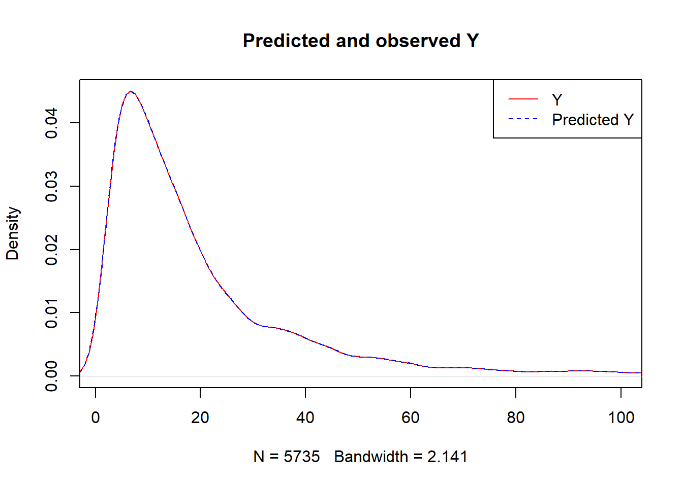

caret::RMSE(predY,Y)

## [1] 0.01255211

What we have done here is we have used the ObsData.matrix data to train our model, and we have used newdata = ObsData.matrix to obtain prediction.

When we use same data for training and obtaining prediction, often the predictions are highly optimistic (RMSE is unrealistically low for future predictions), and we call this a over-fitting problem.

One way to deal with this problem is called Cross-validation.

3.1.2 Cross-validation

Cross-validation means

splitting the data into
- training data
- testing data

In each iteration: (1) Fitting models in training data (2) obtaining prediction \(\hat{Y}\) in test data (3) obtain all RMSEs from each iteration, and (4) average all RMSEs.

Cross validation from [wiki](https://en.wikipedia.org/wiki/Cross-validation_(statistics)); training data = used for building model; test data = used for prediction from the model that was built using training data; each iteration = fold

Figure 3.1: Cross validation from wiki; training data = used for building model; test data = used for prediction from the model that was built using training data; each iteration = fold

3.1.2.1 Cross-validation using caret

We use caret package to do cross-validation.

caret is a general framework package for machine learning that can also incorporate other ML approaches such as xgboost.

require(caret)
set.seed(123)
X_ObsData.matrix <- xgb.DMatrix(ObsData.matrix)
Y_ObsData <- ObsData$Y

Below we define \(K = 3\) for cross-validation. Ideally for a sample size close to \(n=5,000\), we would select \(K=10\), but for learning / demonstration / computational time-saving purposes, we just use \(K = 3\).

xgb_trcontrol = trainControl(
  method = "cv",
  number = 3,  
  allowParallel = TRUE,
  verboseIter = FALSE,
  returnData = FALSE
)

3.1.2.2 Fine tuning

One of the advantages of caret framework is that, it also allows checking the impact of various parameters (can do fine tuning).

For example,

for interaction depth, we previously use max.depth = 10. That means \(covariate^{10}\) polynomial.
We could also check if other interaction depth choices (such as \(covariate^{2}\) or \(covariate^{4}\)) would be better in terms of honest predictions.

xgbGrid <- expand.grid(
  nrounds = 100, 
  max_depth = seq(2,10,2),
  eta = 1,
  gamma = 0,
  colsample_bytree = 0.1,
  min_child_weight = 2,
  subsample = 0.5 
)

3.1.2.3 Fit model with CV

once we set

resampling or cross-validation settings
parameter grid

we can fit the model:

fit.xgb <- train(
  X_ObsData.matrix, Y_ObsData,  
  trControl = xgb_trcontrol,
  method = "xgbTree",
  tuneGrid = xgbGrid,
  verbose = FALSE
)
fit.xgb

## eXtreme Gradient Boosting 
## 
## No pre-processing
## Resampling: Cross-Validated (3 fold) 
## Summary of sample sizes: 3822, 3824, 3824 
## Resampling results across tuning parameters:
## 
##   max_depth  RMSE      Rsquared     MAE     
##    2         28.87561  0.020524186  19.08176
##    4         38.88354  0.007198028  28.08175
##    6         49.62373  0.002200636  37.69929
##    8         54.86092  0.004255366  42.40188
##   10         57.13972  0.001224946  44.15276
## 
## Tuning parameter 'nrounds' was held constant at a value of 100
## Tuning
##  held constant at a value of 2
## Tuning parameter 'subsample' was held
##  constant at a value of 0.5
## RMSE was used to select the optimal model using the smallest value.
## The final values used for the model were nrounds = 100, max_depth = 2, eta =
##  1, gamma = 0, colsample_bytree = 0.1, min_child_weight = 2 and subsample = 0.5.

Based on the loss function (say, RMSE) it automatically chose the best tuning parameter set:

fit.xgb$bestTune$max_depth

## [1] 2

predY <- predict(fit.xgb, newdata = ObsData.matrix)
plot(density(Y), 
     col = "red", 
     main = "Predicted and observed Y",
     xlim = c(1,100))  
legend("topright", 
       c("Y","Predicted Y"), 
       lty = c(1,2), 
       col = c("red","blue"))
lines(density(predY), col = "blue", lty = 2)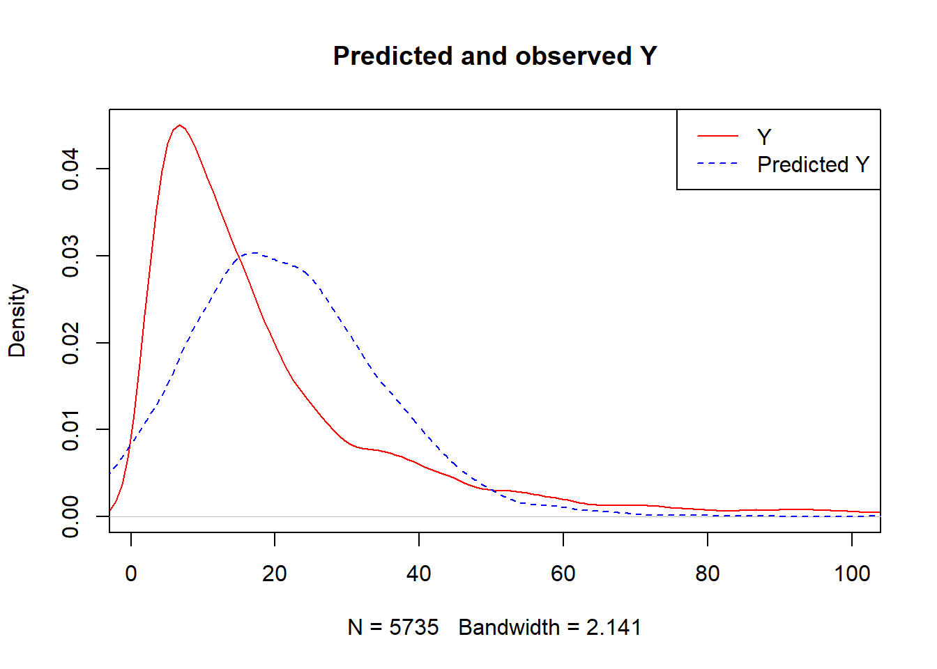

caret::RMSE(predY,Y)

## [1] 24.35099

3.1.3 G-comp step 2: Extract outcome prediction as if everyone is treated

ObsData.matrix.A1 <- ObsData.matrix 
ObsData.matrix.A1[,"A"] <- 1
ObsData$Pred.Y1 <- predict(fit.xgb, newdata = ObsData.matrix.A1)
summary(ObsData$Pred.Y1)

##    Min. 1st Qu.  Median    Mean 3rd Qu.    Max. 
##  -33.15   14.87   23.09   23.89   31.78  131.48

3.1.4 G-comp step 3: Extract outcome prediction as if everyone is untreated

ObsData.matrix.A0 <- ObsData.matrix
ObsData.matrix.A0[,"A"] <- 0
ObsData$Pred.Y0 <- predict(fit.xgb, newdata = ObsData.matrix.A0)
summary(ObsData$Pred.Y0)

##    Min. 1st Qu.  Median    Mean 3rd Qu.    Max. 
##  -37.31   10.72   18.96   19.78   27.69  127.31

3.1.5 G-comp step 4: Treatment effect estimate

ObsData$Pred.TE <- ObsData$Pred.Y1 - ObsData$Pred.Y0

Mean value of predicted treatment effect

TE1 <- mean(ObsData$Pred.TE)
TE1

## [1] 4.110383

summary(ObsData$Pred.TE)

##    Min. 1st Qu.  Median    Mean 3rd Qu.    Max. 
##  -5.494   4.165   4.165   4.110   4.165   9.339

Notice that the mean is slightly different than the parametric G-computation method.

3.2 G-comp using regularized methods

3.2.1 A regularized model

LASSO is a regularized method. One of the uses of these methods is “variable selection” or addressing concerns of multicollinearity.

Let us use this method to fit our data.

We are again using cross-validation here, and we chose \(K=3\).

require(glmnet)
Y <-ObsData$Y
ObsData.matrix <- model.matrix(out.formula, data = ObsData)
fit4 <-  cv.glmnet(x = ObsData.matrix, 
                y = Y,
                alpha = 1,
                nfolds = 3,
                relax=TRUE)

3.2.2 G-comp step 2: Extract outcome prediction as if everyone is treated

ObsData.matrix.A1 <- ObsData.matrix 
ObsData.matrix.A1[,"A"] <- 1
ObsData$Pred.Y1 <- predict(fit4, newx = ObsData.matrix.A1,
                           s = "lambda.min")
summary(ObsData$Pred.Y1)

##    lambda.min    
##  Min.   :-30.41  
##  1st Qu.: 19.53  
##  Median : 23.95  
##  Mean   : 23.24  
##  3rd Qu.: 27.26  
##  Max.   : 38.14

3.2.3 G-comp step 3: Extract outcome prediction as if everyone is untreated

ObsData.matrix.A0 <- ObsData.matrix
ObsData.matrix.A0[,"A"] <- 0
ObsData$Pred.Y0 <- predict(fit4, newx = ObsData.matrix.A0,
                           s = "lambda.min")
summary(ObsData$Pred.Y0)

##    lambda.min    
##  Min.   :-33.13  
##  1st Qu.: 16.81  
##  Median : 21.23  
##  Mean   : 20.52  
##  3rd Qu.: 24.54  
##  Max.   : 35.42

3.2.4 G-comp step 4: Treatment effect estimate

ObsData$Pred.TE <- ObsData$Pred.Y1 - ObsData$Pred.Y0

Mean value of predicted treatment effect

TE2 <- mean(ObsData$Pred.TE)
TE2

## [1] 2.719739

summary(ObsData$Pred.TE)

##    lambda.min  
##  Min.   :2.72  
##  1st Qu.:2.72  
##  Median :2.72  
##  Mean   :2.72  
##  3rd Qu.:2.72  
##  Max.   :2.72

Notice that the mean is very similar to the parametric G-computation method.

3.3 G-comp using SuperLearner

SuperLearner is an ensemble ML technique, that uses cross-validation to find a weighted combination of estimates provided by different candidate learners (that help predict).

There exists many candidate learners. Here we are using a combination of
- linear regression
- Regularized regression (lasso)
- gradient boosting (tree based)

3.3.1 Steps

Step 1	Identify candidate learners
Step 2	Choose Cross-validation K
Step 3	Select loss function for meta learner
Step 4	Find SL prediction: (1) Discrete SL (2) Ensamble SL

3.3.1.1 Identify candidate learners

Choose variety of candidate learners
- parametric (linear or logistic regression)
- regularized (LASSO, ridge, elasticnet)
- stepwise
- non-parametric
- transformation (SVM, NN)
- tree based (bagging, boosting)
- smoothing or spline (gam)
tune the candidate learners for better performance
- tree depth
- tune regularization parameters
- variable selection

SL.library.chosen=c("SL.glm", "SL.glmnet", "SL.xgboost")

SuperLearner is an ensemble learning method. Let us use this one to fit the data first.

3.3.1.2 Choose Cross-validation K

To combat against optimism, we use cross-validation. SuperLearner first splits the data according to chosen \(K\) fold for the cross-validation.

cvControl.chosen = list(V = 3)

3.3.1.3 Select loss function for meta learner and estimate risk

The goal is to minimize the estimated risk (i.e., minimize the difference of \(Y\) and \(\hat{Y}\)) that comes out of a model.

We can chose a (non-negative) least squares loss function for the meta learner (explained below):

loss.chosen = "method.NNLS"

3.3.1.4 Find SL prediction

We first fit the super learner:

require(SuperLearner)
ObsData.noY <- dplyr::select(ObsData, !Y)
fit.sl <- SuperLearner(Y=ObsData$Y, 
                       X=ObsData.noY, 
                       cvControl = cvControl.chosen,
                       SL.library=SL.library.chosen,
                       method=loss.chosen,
                       family="gaussian")

We can also obtain the predictions from each candidate learners.

all.pred <- predict(fit.sl, type = "response")
Yhat <- all.pred$library.predict
head(Yhat)

##   SL.glm_All SL.glmnet_All SL.xgboost_All
## 1   14.61647      14.57121      14.890952
## 2   28.66305      28.96897      42.775368
## 3   24.57800      24.98479      49.592552
## 4   18.70422      19.20871      25.078993
## 5   13.64956      12.18804       8.819989
## 6   22.56895      21.60971      11.892698

We can obtain the \(K\)-fold cross-validated risk estimates for each candidate learners.

fit.sl$cvRisk

##     SL.glm_All  SL.glmnet_All SL.xgboost_All 
##       634.4393       622.8681       737.5505

Once we have the performance measures and predictions from candidate learners, we could go one of two routes here

3.3.1.4.1 Discrete SL

Get measure of performance from all folds are averaged, and choose the best one. The prediction from the chosen learners are then used.

glmnet has the lowest cross-validated risk

lowest.risk.learner <- names(which(
  fit.sl$cvRisk == min(fit.sl$cvRisk)))
lowest.risk.learner

## [1] "SL.glmnet_All"

as.matrix(head(Yhat[,lowest.risk.learner]), 
          ncol=1)

##       [,1]
## 1 14.57121
## 2 28.96897
## 3 24.98479
## 4 19.20871
## 5 12.18804
## 6 21.60971

3.3.1.4.2 Ensamble SL

Here are the first 6 rows from the candidate learner predictions:

head(Yhat)

##   SL.glm_All SL.glmnet_All SL.xgboost_All
## 1   14.61647      14.57121      14.890952
## 2   28.66305      28.96897      42.775368
## 3   24.57800      24.98479      49.592552
## 4   18.70422      19.20871      25.078993
## 5   13.64956      12.18804       8.819989
## 6   22.56895      21.60971      11.892698

fit a meta learner (optimal weighted combination; below is a simplified description)

using
- linear regression (without intercept, but could produce -ve coefs) or
- preferably non-negative least squares for
\(Y_{obs}\) \(\sim\) \(\hat{Y}_{SL.glm}\) + \(\hat{Y}_{SL.glmnet}\) + \(\hat{Y}_{SL.xgboost}\).
Obtain the regression coefs \(\mathbf{\beta}\) = (\(\beta_{SL.glm}\), \(\beta_{SL.glmnet}\), \(\beta_{SL.xgboost}\)) for each \(\hat{Y}\),
scale them to 1
- \(\mathbf{\beta_{scaled}}\) = \(\mathbf{\beta}\) / \(\sum_{i=1}^3{\mathbf{\beta}}\);
- so that the sum of scaled coefs = 1
Scaled coefficients \(\mathbf{\beta_{scaled}}\) represents the value / importance of the corresponding candidate learner.

Scaled coefs

fit.sl$coef

##     SL.glm_All  SL.glmnet_All SL.xgboost_All 
##     0.00000000     0.93740912     0.06259088

sum(fit.sl$coef)

## [1] 1

Hence, in creating superlearner prediction column,

Linear regression has no contribution
lasso has majority contribution
gradient boosting of tree has some minimal contribution

A new prediction column is produced based on the fitted values from this meta regression.

You can simply multiply these coefs to the predictions from candidate learners, and them sum them to get ensable SL. Here are the first 6 values:

SL.ens <- t(t(Yhat)*fit.sl$coef)
head(SL.ens)

##   SL.glm_All SL.glmnet_All SL.xgboost_All
## 1          0      13.65919      0.9320378
## 2          0      27.15577      2.6773480
## 3          0      23.42097      3.1040416
## 4          0      18.00642      1.5697163
## 5          0      11.42518      0.5520509
## 6          0      20.25714      0.7443745

as.matrix(head(rowSums(SL.ens)), ncol = 1)

##       [,1]
## 1 14.59123
## 2 29.83312
## 3 26.52501
## 4 19.57614
## 5 11.97723
## 6 21.00152

Alternatively, you can get them directly from the package: here are the first 6 values

head(all.pred$pred)

##       [,1]
## 1 14.59123
## 2 29.83312
## 3 26.52501
## 4 19.57614
## 5 11.97723
## 6 21.00152

The last column is coming from Ensamble SL.

3.3.2 G-comp step 2: Extract outcome prediction as if everyone is treated

We are going to use Ensamble SL predictions in the following calculations. If you wanted to use discrete SL predictions instead, that would be fine too.

ObsData.noY$A <- 1
ObsData$Pred.Y1 <- predict(fit.sl, newdata = ObsData.noY,
                           type = "response")$pred

## Warning in predict.lm(object, newdata, se.fit, scale = 1, type = if (type == :
## prediction from a rank-deficient fit may be misleading

summary(ObsData$Pred.Y1)

##        V1        
##  Min.   :-31.15  
##  1st Qu.: 18.70  
##  Median : 23.40  
##  Mean   : 22.75  
##  3rd Qu.: 27.09  
##  Max.   : 58.48

3.3.3 G-comp step 3: Extract outcome prediction as if everyone is untreated

ObsData.noY$A <- 0
ObsData$Pred.Y0 <- predict(fit.sl, newdata = ObsData.noY,
                           type = "response")$pred

## Warning in predict.lm(object, newdata, se.fit, scale = 1, type = if (type == :
## prediction from a rank-deficient fit may be misleading

summary(ObsData$Pred.Y0)

##        V1        
##  Min.   :-33.10  
##  1st Qu.: 16.76  
##  Median : 21.50  
##  Mean   : 20.83  
##  3rd Qu.: 25.18  
##  Max.   : 55.86

3.3.4 G-comp step 4: Treatment effect estimate

ObsData$Pred.TE <- ObsData$Pred.Y1 - ObsData$Pred.Y0

Mean value of predicted treatment effect

TE3 <- mean(ObsData$Pred.TE)
TE3

## [1] 1.914702

summary(ObsData$Pred.TE)

##        V1       
##  Min.   :1.099  
##  1st Qu.:1.849  
##  Median :1.907  
##  Mean   :1.915  
##  3rd Qu.:1.976  
##  Max.   :2.991

3.3.5 Additional details for SL

3.3.5.1 Choice of K

simplest cross-validation splits the data into \(K=2\) parts, but can go higher.
- select \(K\) judiciously
  - large sample size means small \(K\) may be adequate
    - for \(n \lt 10,000\) consider \(K=3\)
    - for \(n \lt 500\) consider \(K=20\)
  - smaller sample size means larger \(K\) may be necessary
    - for \(n \lt 30\) consider leave 1 out

3.3.5.2 Alternative to CV

other similar algorithms such as cross-fitting had been shown to have better performances

3.3.5.3 Rare outcome

for rare outcomes, consider using stratification to attempt to maintain training and test sample ratios the same

3.3.5.4 Dependant sample

if data is clustered and not independent and identically distributed, use ID for the cluster

3.3.5.5 Choice of meta learner method

It is easy to show that, depending on the choice of meta-learners, the coefficients of the meta learners can be slightly different.

fit.sl2 <- recombineSL(fit.sl, Y = Y, 
                       method = "method.NNLS2")
fit.sl2$coef

##     SL.glm_All  SL.glmnet_All SL.xgboost_All 
##     0.00000000     0.93740912     0.06259088

fit.sl2 <- recombineSL(fit.sl, Y = Y, 
                       method = "method.CC_LS")
fit.sl2$coef

##     SL.glm_All  SL.glmnet_All SL.xgboost_All 
##     0.00000000     0.93662601     0.06337399

fit.sl4 <- recombineSL(fit.sl, Y = Y, 
                       method = "method.CC_nloglik")
fit.sl4$coef

##     SL.glm_All  SL.glmnet_All SL.xgboost_All 
##              0              1              0

method.CC_LS is suggested as a good method for continuous outcome
method.CC_nloglik is suggested as a good method for binary outcome

saveRDS(TE1, file = "data/gcompxg.RDS")
saveRDS(TE2, file = "data/gcompls.RDS")
saveRDS(TE3, file = "data/gcompsl.RDS")