Collider
In causal inference, understanding the role of colliders is crucial. A collider is a variable that is a common effect of two or more variables. Adjusting for a collider can introduce bias into your estimates.
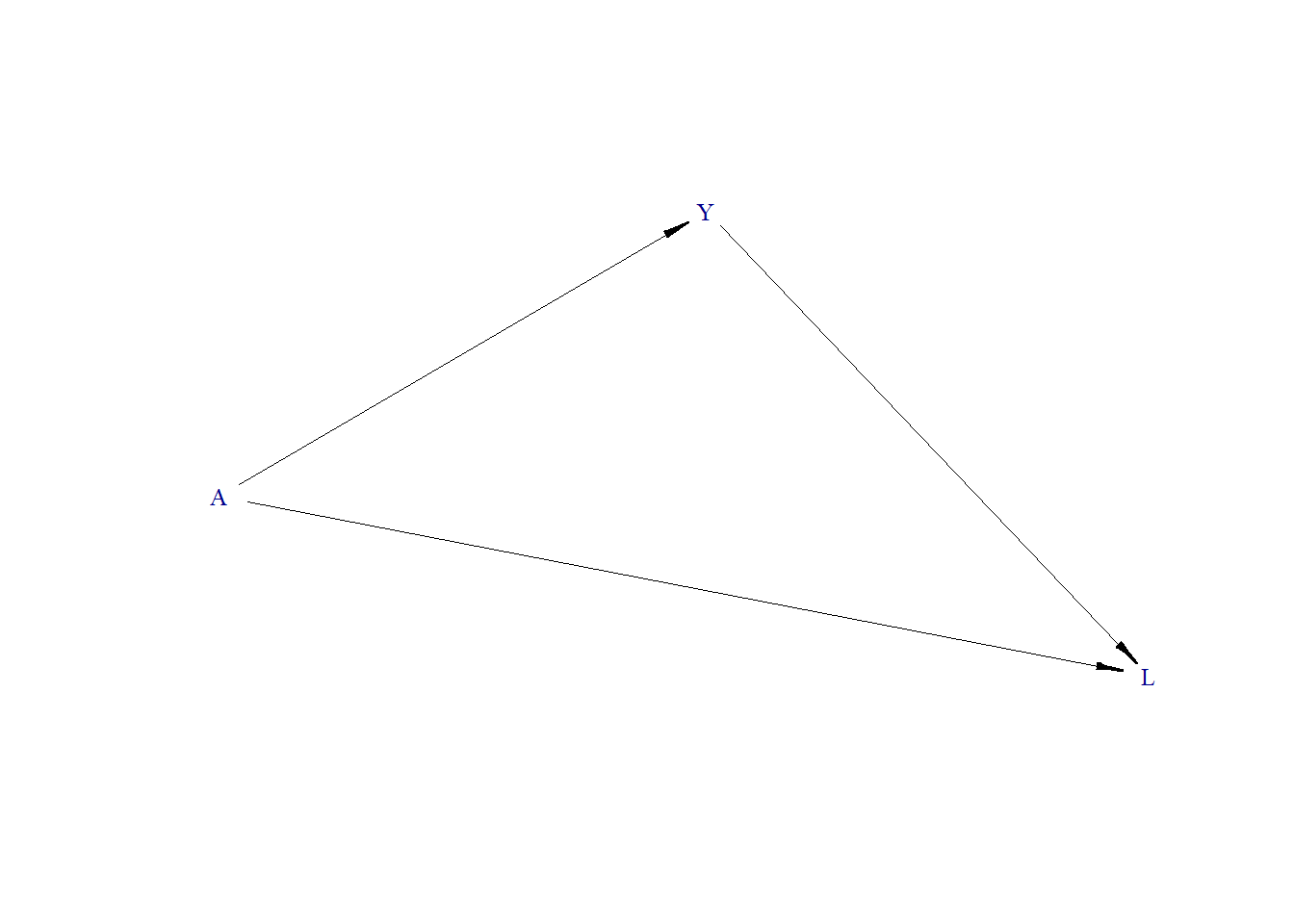
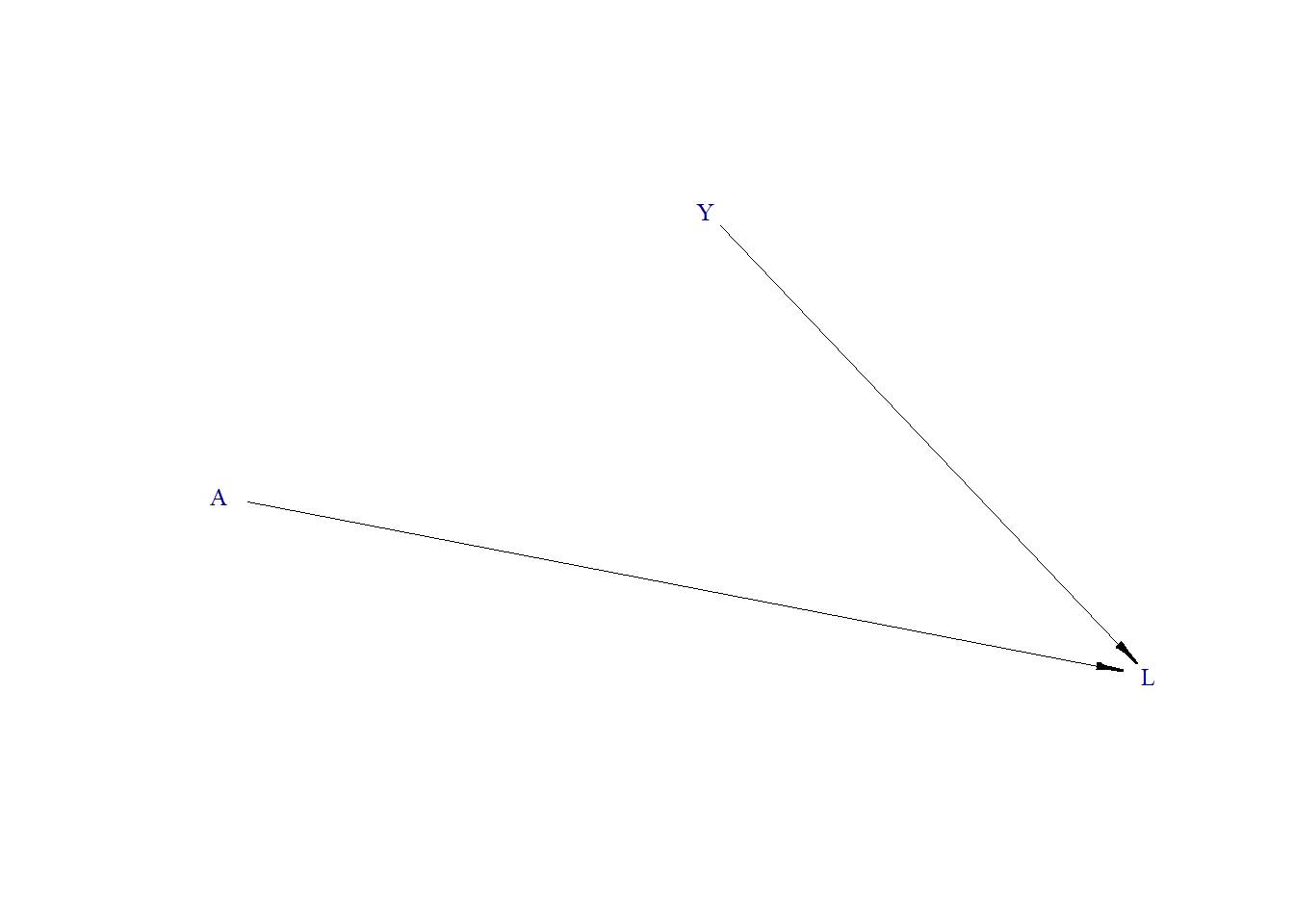
In a DAG, a collider is a variable influenced by two or more other variables. In our case, L is a collider because it is affected by both A (the treatment) and Y (the outcome). When you adjust for a collider like L, you could introduce bias into your estimates, as demonstrated in the examples below.
Let us consider
- L is continuous variable
- A is binary treatment/exposure
- Y is continuous outcome
An example of A could be a genetic variable (e.g., skin color), Y could be an environmental variable (e.g., indoor air pollution), and L could be disease conditions (e.g., number of comorbidities) (detailed expamles here).
Non-null effect
- True treatment effect = 1.3
Data generating process
Generate DAG
Generate data
Estimate effect
When not adjusting for L, we recover the true effect close to 1.3. Adjusting for L introduces bias, making the estimate unreliable.
Null effect
- True treatment effect = 0
Data generating process
Generate DAG
Generate data
Estimate effect
When the true effect is null, not adjusting for L shows an estimate close to zero. Adjusting for L moves the estimate away from the null value, introducing bias.
Note that the bias from adjusting for the collider L does not go away as the sample size grows: collider bias is a structural (asymptotic) bias built into the data-generating process, not a small-sample artifact. Even with 1,000,000 observations the collider-adjusted estimate remains biased, while the unadjusted estimate recovers the true effect.