MCAR tests

MCAR tests are essential tools in the data analysis process. They help researchers understand the nature of missingness in their datasets, guide appropriate imputation strategies, and ensure the validity and reliability of statistical analyses.

MCAR data

In the initial chunk, several packages are loaded. These packages provide functions and tools necessary for the subsequent analysis, including multiple imputation, statistical modeling, and data visualization.

# Load required packages
require(mice)
require(mitools)
require(survey)
require(remotes)
require(simcausal)

Data generating process

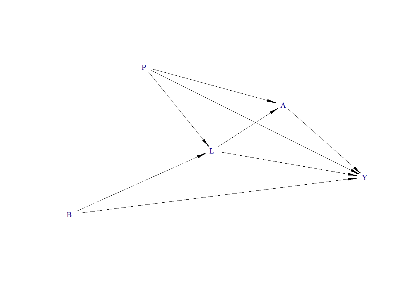
A Directed Acyclic Graph (DAG) is defined, which represents a causal model of how different variables in the dataset relate to each other. This DAG is used to simulate data based on the relationships defined. We generate L as a function of P and B.

require(simcausal)
D <- DAG.empty()
D <- D + 
  node("B", distr = "rnorm", mean = 0, sd = 1) +
  node("P", distr = "rnorm", mean = 0, sd = .7) +
  node("L", distr = "rnorm", mean = 2 + 2 * P + 3 * B, sd = 3) + 
  node("A", distr = "rnorm", mean = 0.5 + L + 2 * P, sd = 1) + 
  node("Y", distr = "rnorm", mean = 1.1 * L + 1.3 * A + B + 2 * P, sd = .5)
Dset <- set.DAG(D)

Generate DAG

The previously defined DAG is visualized, providing a graphical representation of the relationships between variables.

plotDAG(Dset, xjitter = 0.1, yjitter = .9,
        edge_attrs = list(width = 0.5, arrow.width = 0.4, arrow.size = 0.7),
        vertex_attrs = list(size = 12, label.cex = 0.8))

Generate Data

Using the DAG, a dataset is simulated. This dataset will be used for subsequent analysis.

Obs.Data <- sim(DAG = Dset, n = 10000, rndseed = 123)
head(Obs.Data)

Obs.Data.original <- Obs.Data

Randomly set some data to missing

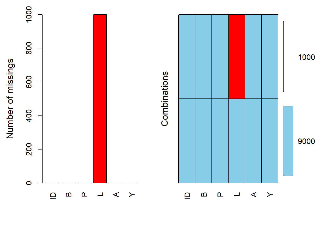
Some values in the dataset are randomly set to missing (i.e., randomly assign some L values to missing). This simulates a scenario where data might be missing completely at random (MCAR).

set.seed(123)
Obs.Data$L[sample(1:length(Obs.Data$L), size = 1000)] <- NA
summary(Obs.Data$L)
#>    Min. 1st Qu.  Median    Mean 3rd Qu.    Max.    NA's 
#> -17.116  -1.096   1.896   1.968   4.996  20.129    1000

The missing data patterns in the dataset are visualized. This helps in understanding which variables have missing values and how they might be related.

require(VIM)
res <- aggr(Obs.Data, plot = FALSE)
plot(res, numbers = TRUE, prop = FALSE)

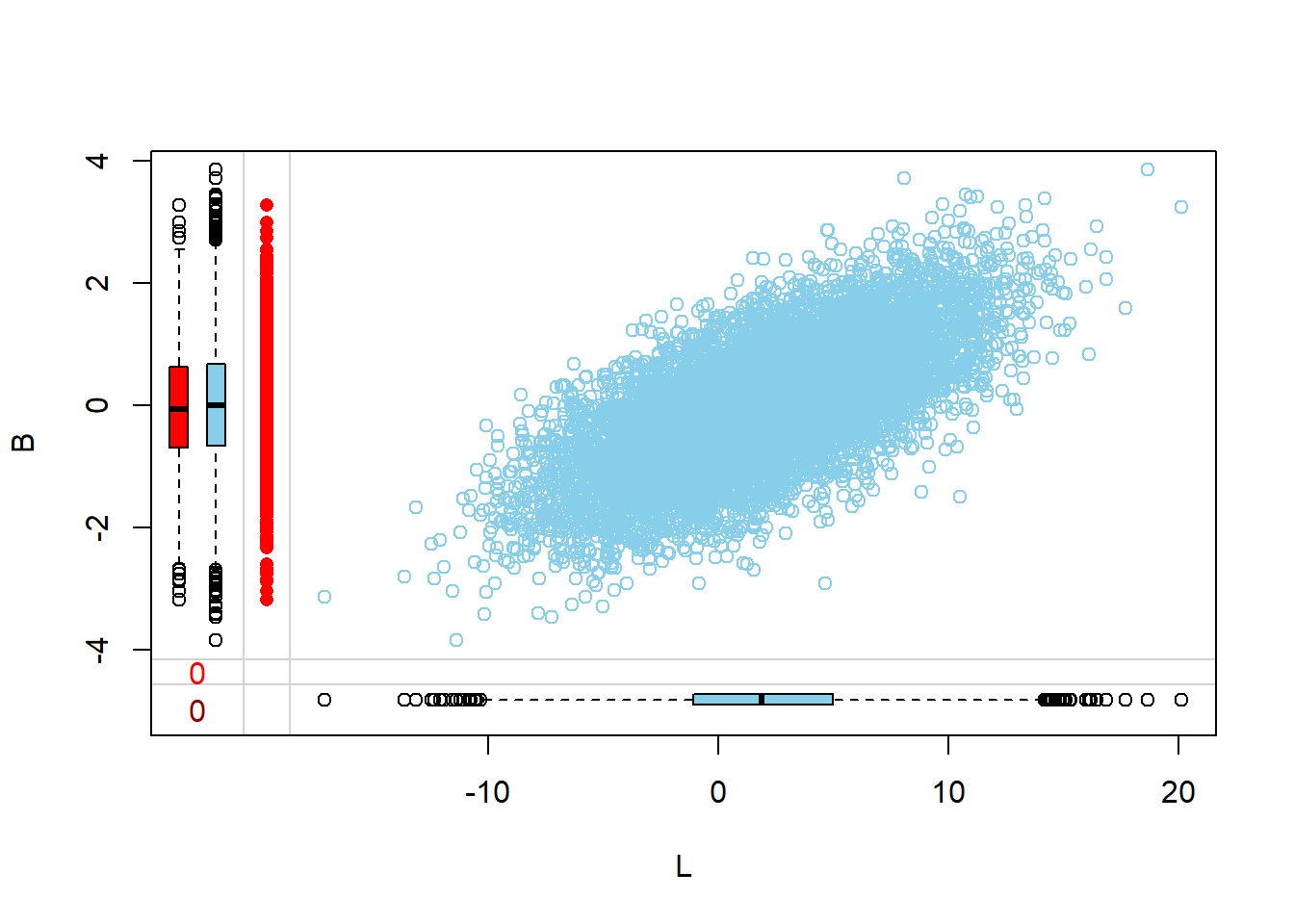
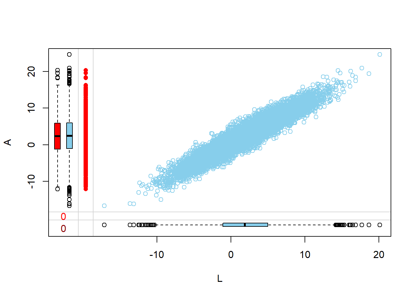
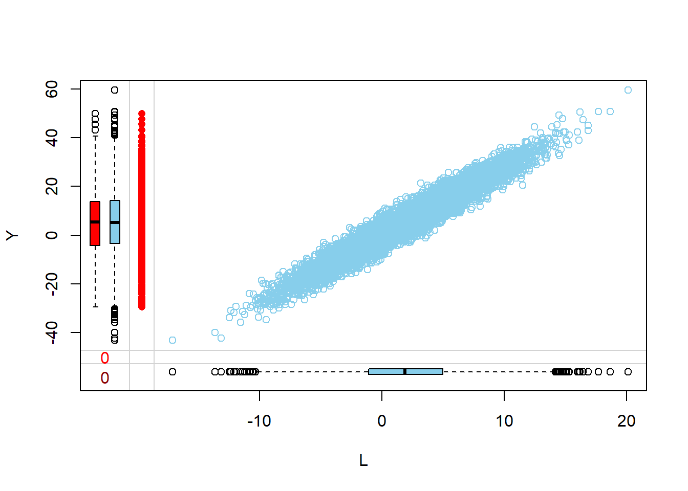
Visualize via margin plots

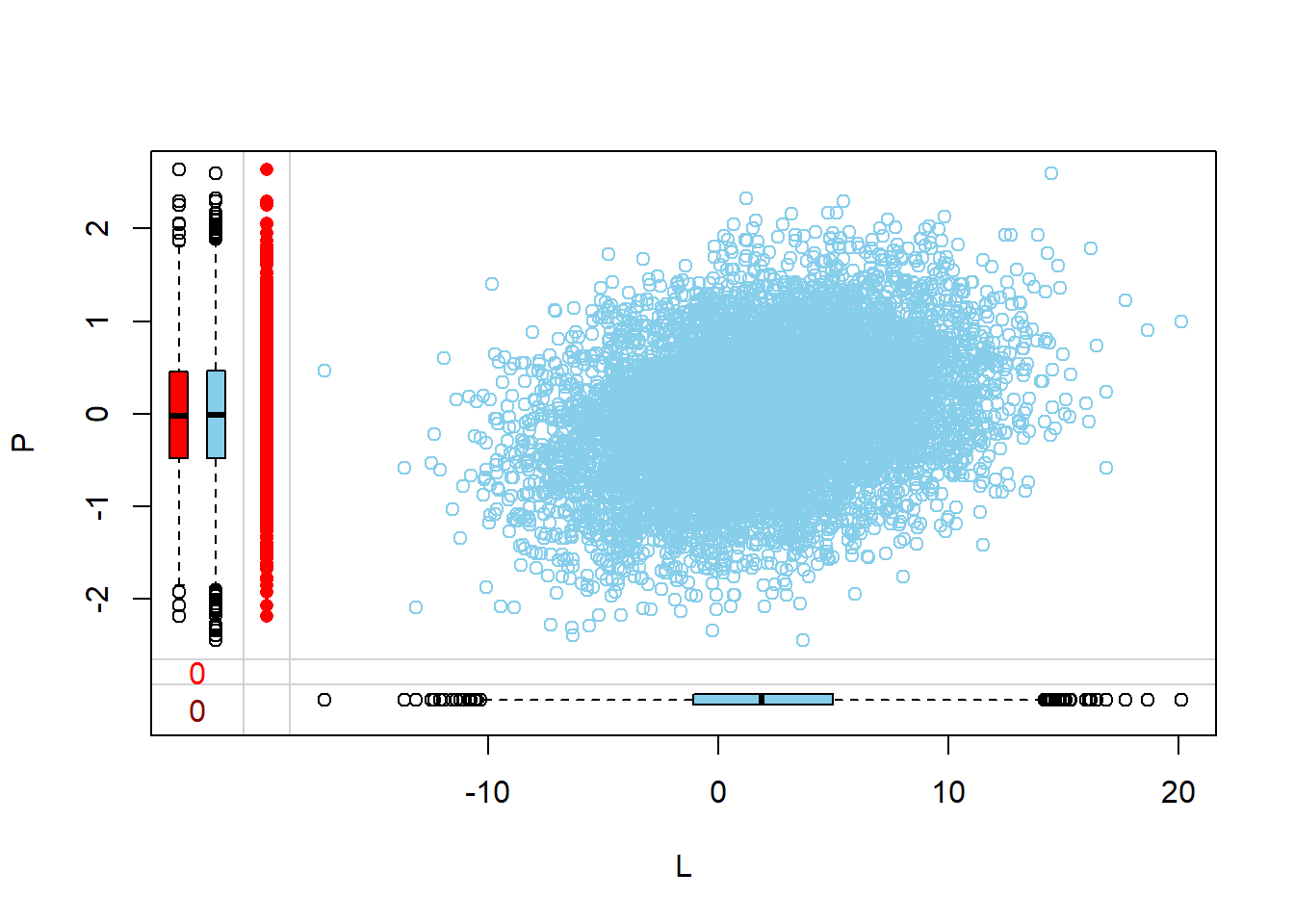
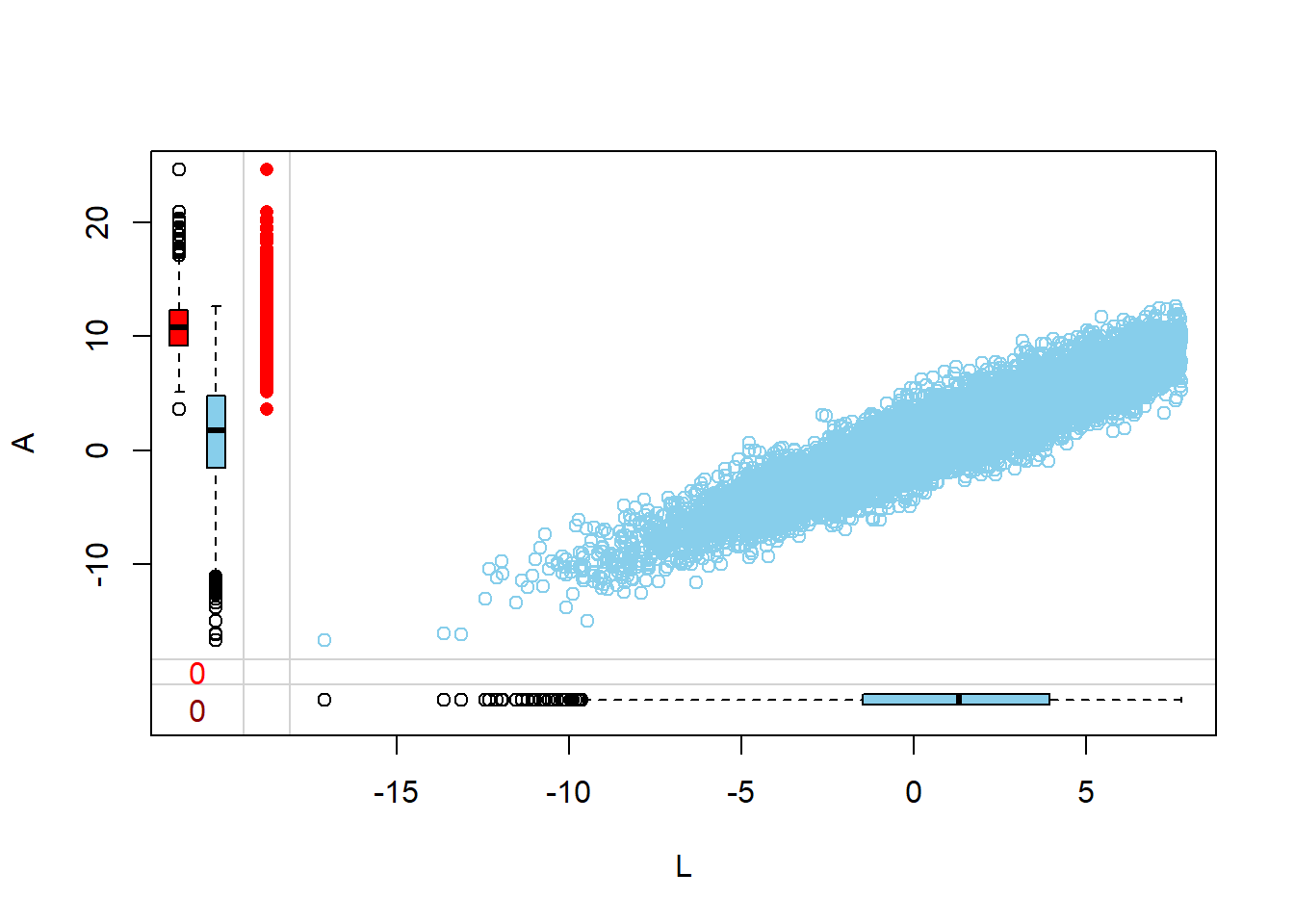
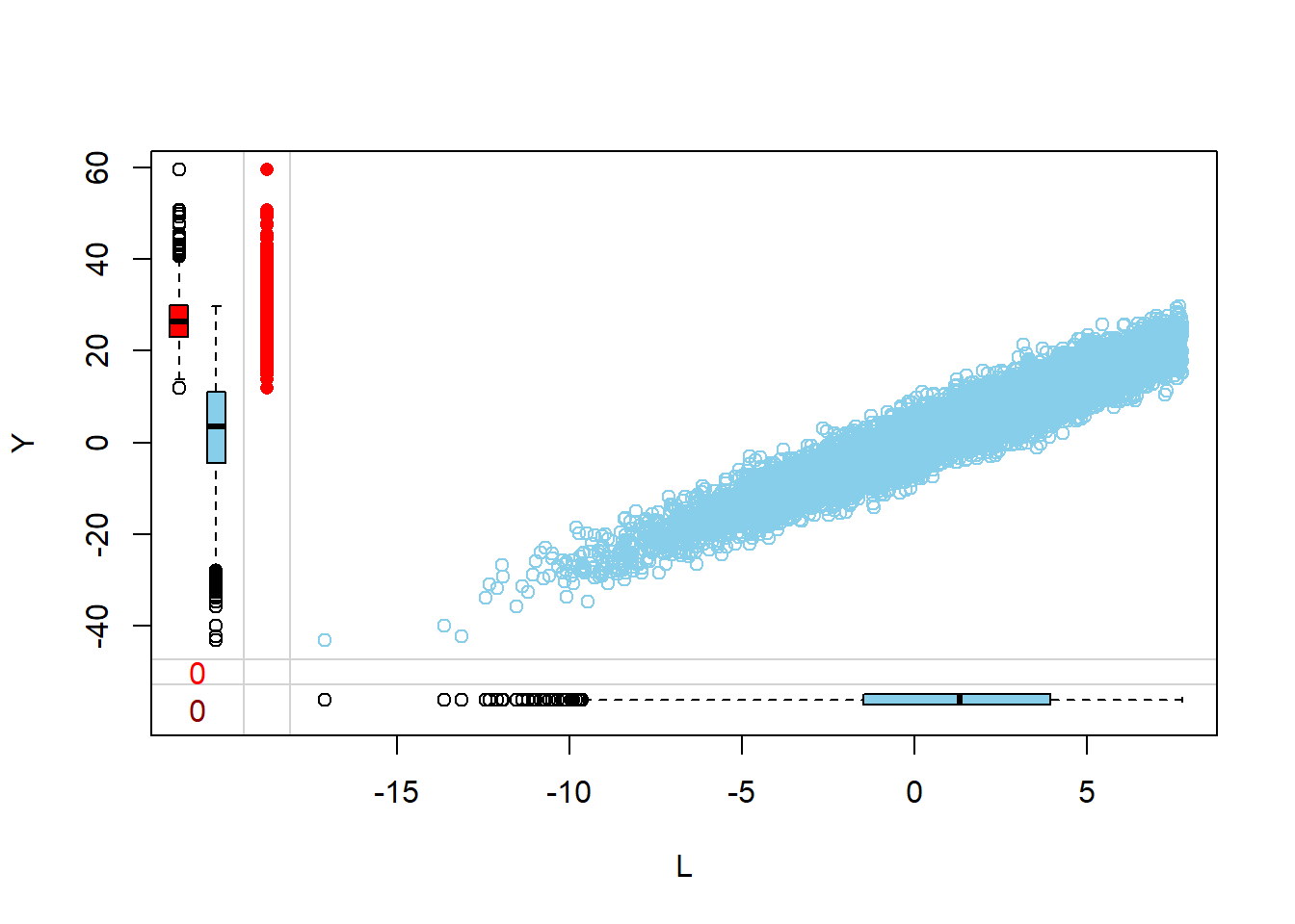
Margin plots are used to compare the distributions of variables when a particular variable is missing versus when it is observed. This provides insights into how missingness might be related to the values of other variables.

The red boxplot depicts the distribution of a variable in the data where L has a missing value.
The blue boxplot depicts the distribution of the values of a variable in the data where L has an observed value.
Same median and spread (range) may mean no difference in the distribution.

marginplot(Obs.Data[,c("L", "P")])

marginplot(Obs.Data[,c("L", "B")])

marginplot(Obs.Data[,c("L", "A")])

marginplot(Obs.Data[,c("L", "Y")])

Little’s MCAR test

A statistical test is conducted to determine if data is missing entirely at random (MCAR). The outcome of this test offers a deeper understanding of the reasons behind the missing data.

Little’s 1988 chi-squared test evaluates if data is MCAR by checking for significant differences in the means of various missing-value patterns (Little 1988). Based on the test’s statistic and p-value, we can infer if the data is MCAR. The null hypothesis for this test is that the data is MCAR.

The essence of this test is to compare means across groups with different missing data patterns. It uses a likelihood ratio test and assumes the data follows a multivariate normal distribution.
If this test is rejected (indicated by a low p-value or a high statistic), it suggests the data might not be MCAR.

However, this test has several limitations (rdrr 2023):

The test doesn’t pinpoint which specific variables don’t adhere to MCAR, meaning it doesn’t highlight potential variables associated with missingness.
It assumes multivariate normality. If this assumption isn’t met, especially with non-normal or categorical variables, the test might not be reliable unless there’s a large sample size.
The test assumes that all missing data patterns have the same covariance matrix. This means it can’t detect deviations from MCAR that are based on covariance, especially if the data is Missing at Random (MAR) or Missing Not at Random (MNAR).
Research has shown that Little’s MCAR test might have low power, especially when few variables don’t follow MCAR, the association between the data and its missingness is weak, or if the data is MNAR.
The test can only reject the MCAR assumption but can’t confirm it. A non-significant result doesn’t necessarily confirm that the data is MCAR.
Even if the test result is significant, it doesn’t rule out the possibility of the data being MNAR.

require(naniar)
mcar_test(Obs.Data)


require(misty)
na.test(Obs.Data)
#>  Little's MCAR Test
#> 
#>       n nIncomp nPattern chi2 df  pval 
#>   10000    1000        2 2.60  5 0.761

MCAR and normality test

Hawkins, in 1981, introduced a method to assess both multivariate normality and the consistency in variances, known as homoscedasticity. This method not only checks for consistent variances but also for mean equality (Hawkins 1981).

In 2010, Jamshidian and Jalal suggested a technique to compare covariances among groups with the same missing data patterns. They utilized the Hawkins test for data assumed to be normal and a non-parametric approach for other data types (Jamshidian and Jalal 2010).

The following package (Jamshidian and Jalal 2010) tests multivariate normality and homoscedasticity in the context of missing data.

#library(devtools)
#install_github("cran/MissMech")
library(MissMech)
test.result <- TestMCARNormality(data = Obs.Data)
test.result
#> Call:
#> TestMCARNormality(data = Obs.Data)
#> 
#> Number of Patterns:  2 
#> 
#> Total number of cases used in the analysis:  10000 
#> 
#>  Pattern(s) used:
#>           ID   B   P    L   A   Y   Number of cases
#> group.1    1   1   1   NA   1   1              1000
#> group.2    1   1   1    1   1   1              9000
#> 
#> 
#>     Test of normality and Homoscedasticity:
#>   -------------------------------------------
#> 
#> Hawkins Test:
#> 
#>     P-value for the Hawkins test of normality and homoscedasticity:  1.749746e-15 
#> 
#>     Either the test of multivariate normality or homoscedasticity (or both) is rejected.
#>     Provided that normality can be assumed, the hypothesis of MCAR is 
#>     rejected at 0.05 significance level. 
#> 
#> Non-Parametric Test:
#> 
#>     P-value for the non-parametric test of homoscedasticity:  0.4019219 
#> 
#>     Reject Normality at 0.05 significance level.
#>     There is not sufficient evidence to reject MCAR at 0.05 significance level.
summary(test.result)
#> 
#> Number of imputation:  1 
#> 
#> Number of Patterns:  2 
#> 
#> Total number of cases used in the analysis:  10000 
#> 
#>  Pattern(s) used:
#>           ID   B   P    L   A   Y   Number of cases
#> group.1    1   1   1   NA   1   1              1000
#> group.2    1   1   1    1   1   1              9000
#> 
#> 
#>     Test of normality and Homoscedasticity:
#>   -------------------------------------------
#> 
#> Hawkins Test:
#> 
#>     P-value for the Hawkins test of normality and homoscedasticity:  1.749746e-15 
#> 
#> Non-Parametric Test:
#> 
#>     P-value for the non-parametric test of homoscedasticity:  0.4019219

png("E:/GitHub/EpiMethods/Images/missingdata/boxplot.png", width = 600, height = 600)
boxplot(test.result)
dev.off()

boxplot(test.result)

Non-MCAR data

Set some data to missing based on a rule

In this section, the original dataset is restored. Then, for a specific column, any value greater than a certain threshold is set to ‘missing’. A summary of this column is then provided to understand the distribution of missing values.

Obs.Data <- Obs.Data.original
Obs.Data$L[Obs.Data$L > 7.79] <- NA
summary(Obs.Data$L)
#>    Min. 1st Qu.  Median    Mean 3rd Qu.    Max.    NA's 
#> -17.116  -1.482   1.330   1.050   3.954   7.787    1035

The dataset’s missing data patterns are visualized. This visualization helps in understanding which data points are missing and their distribution across the dataset.

res <- aggr(Obs.Data, plot = FALSE)
plot(res, numbers = TRUE, prop = FALSE)

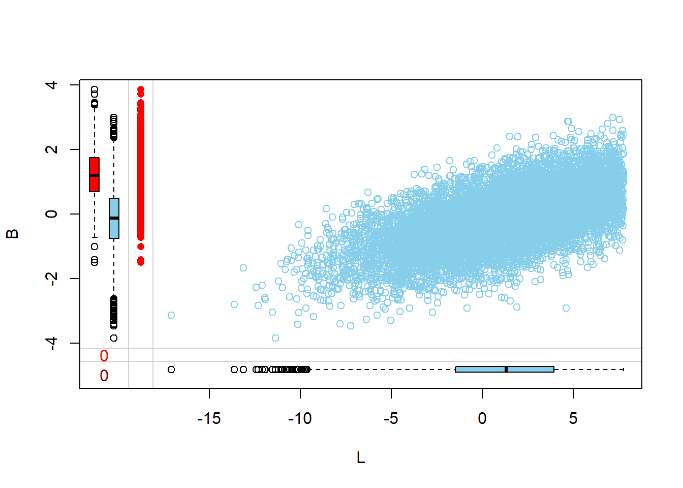
Visualize via margin plots

Margin plots are used to visualize the relationship between two variables, especially when one of them has missing values. Here, the relationship of a specific column with missing values is visualized against other columns in the dataset. This helps in understanding how the missingness in one variable might relate to other variables.

marginplot(Obs.Data[,c("L", "P")])

marginplot(Obs.Data[,c("L", "B")])

marginplot(Obs.Data[,c("L", "A")])

marginplot(Obs.Data[,c("L", "Y")])

Little’s MCAR test

Little’s MCAR test is applied to the dataset to check if the data is missing completely at random. This test provides a statistic and a p-value to determine the nature of missingness in the data.

mcar_test(Obs.Data)

na.test(Obs.Data)
#>  Little's MCAR Test
#> 
#>       n nIncomp nPattern    chi2 df  pval 
#>   10000    1035        2 3511.08  5 0.000

MCAR and normality test

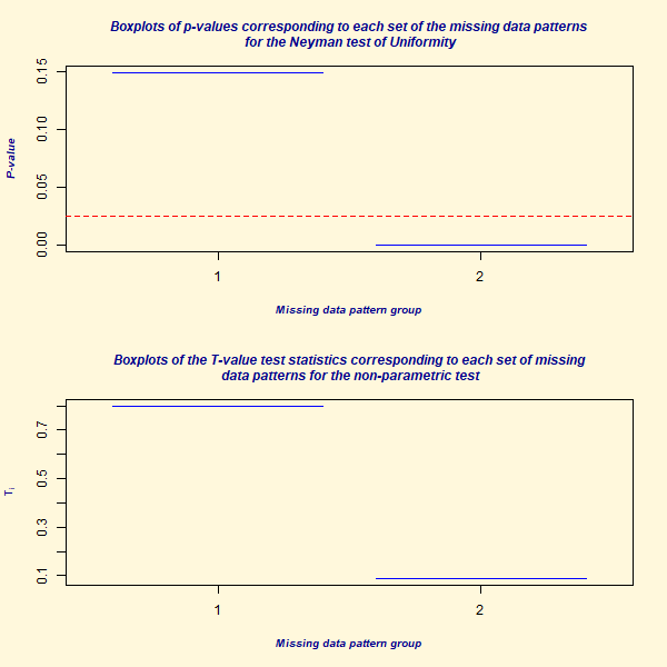
A test is conducted to check if the data follows a multivariate normal distribution and if the variances across different groups are consistent (homoscedasticity). The results of this test, along with a summary and a boxplot visualization, are provided to understand the distribution and characteristics of the data.

test.result <- TestMCARNormality(data = Obs.Data)
test.result
#> Call:
#> TestMCARNormality(data = Obs.Data)
#> 
#> Number of Patterns:  2 
#> 
#> Total number of cases used in the analysis:  10000 
#> 
#>  Pattern(s) used:
#>           ID   B   P    L   A   Y   Number of cases
#> group.1    1   1   1    1   1   1              8965
#> group.2    1   1   1   NA   1   1              1035
#> 
#> 
#>     Test of normality and Homoscedasticity:
#>   -------------------------------------------
#> 
#> Hawkins Test:
#> 
#>     P-value for the Hawkins test of normality and homoscedasticity:  2.401873e-30 
#> 
#>     Either the test of multivariate normality or homoscedasticity (or both) is rejected.
#>     Provided that normality can be assumed, the hypothesis of MCAR is 
#>     rejected at 0.05 significance level. 
#> 
#> Non-Parametric Test:
#> 
#>     P-value for the non-parametric test of homoscedasticity:  0 
#> 
#>     Hypothesis of MCAR is rejected at  0.05 significance level.
#>     The multivariate normality test is inconclusive.
summary(test.result)
#> 
#> Number of imputation:  1 
#> 
#> Number of Patterns:  2 
#> 
#> Total number of cases used in the analysis:  10000 
#> 
#>  Pattern(s) used:
#>           ID   B   P    L   A   Y   Number of cases
#> group.1    1   1   1    1   1   1              8965
#> group.2    1   1   1   NA   1   1              1035
#> 
#> 
#>     Test of normality and Homoscedasticity:
#>   -------------------------------------------
#> 
#> Hawkins Test:
#> 
#>     P-value for the Hawkins test of normality and homoscedasticity:  2.401873e-30 
#> 
#> Non-Parametric Test:
#> 
#>     P-value for the non-parametric test of homoscedasticity:  0

png("E:/GitHub/EpiMethods/Images/missingdata/boxplot1.png", width = 600, height = 600)
boxplot(test.result)
dev.off()

boxplot(test.result)

Hawkins, Douglas M. 1981. “A New Test for Multivariate Normality and Homoscedasticity.” Technometrics 23 (1): 105–10.

Jamshidian, Mortaza, and Siavash Jalal. 2010. “Tests of Homoscedasticity, Normality, and Missing Completely at Random for Incomplete Multivariate Data.” Psychometrika 75 (4): 649–74.

Little, Roderick JA. 1988. “A Test of Missing Completely at Random for Multivariate Data with Missing Values.” Journal of the American Statistical Association 83 (404): 1198–1202.

rdrr. 2023. “Na.test: Little’s Missing Completely at Random (MCAR) Test.” https://rdrr.io/cran/misty/man/na.test.html.