Causal question-2
Working with a causal question using NHANES
We are interested in exploring the relationship between diabetes (binary exposure variable defined as whether the doctor ever told the participant has diabetes) and cholesterol (binary outcome variable). Following the book-wide convention, the cholesterol outcome is coded as 1 = desirable cholesterol (total cholesterol < 200 mg/dL) and 0 otherwise, so the modelled event is desirable cholesterol. Below is the PICOT:
| PICOT element | Description |
|---|---|
| P | US adults |
| I | Diabetes |
| C | No diabetes |
| O | Desirable cholesterol (< 200 mg/dL) |
| T | 2017–2018 |
First, we will prepare the analytic dataset from NHANES 2017–2018.
Second, we will work with subset of data to assess the association between diabetes and cholesterol, and to get proper SE and 95% CI for the estimate. We emphasize the correct usage of the survey’s design features (correct handling of survey design elements, such as stratification, clustering, and weighting) to obtain accurate population-level estimates.
Steps for creating analytic dataset
We will combine multiple components (e.g., demographic, blood pressure) using the unique identifier to create our analytic dataset.
Within NHANES datasets in a given cycle, each sampled person has an unique identifier sequence number (variable SEQN).
Download and Subsetting to retain only the useful variables
Search literature for the relevant variables, and then see if some of them are available in the NHANES data.
Peters, Fabian, and Levy (2014)
An an example, let us assume that variables listed in the following figures are known to be useful. Then we will try to indentify, in which NHANES component we have these variables.
Refer to the earlier chapter to get a more detailed understanding of how we search for variables within NHANES.
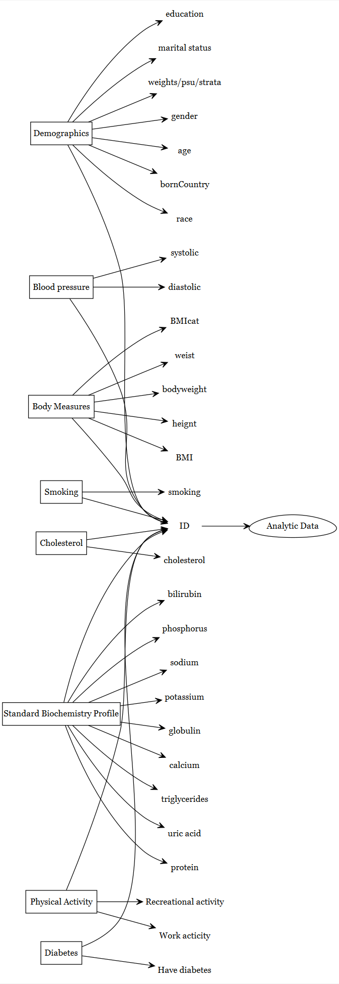
NHANES Data Components:
- Demographic (variables like age, gender, income, etc.)
- Blood Pressure (Diastolic and Systolic pressure)
- Body Measures (BMI, Waist Circumference, etc.)
- Smoking Status (Current smoker or not)
- Cholesterol (Total cholesterol in different units)
- Biochemistry Profile (Triglycerides, Uric acid, etc.)
- Physical Activity (Vigorous work and recreational activities)
- Diabetes (Whether the respondent has been told by a doctor that they have diabetes)
Demographic component:
demo <- nhanes('DEMO_J') # Both males and females 0 YEARS - 150 YEARS
demo <- demo[c("SEQN", # Respondent sequence number
                 "RIAGENDR", # gender
                 "RIDAGEYR", # Age in years at screening
                 "DMDBORN4", # Country of birth
                 "RIDRETH3", # Race/Hispanic origin w/ NH Asian
                 "DMDEDUC3", # Education level - Children/Youth 6-19
                 "DMDEDUC2", # Education level - Adults 20+
                 "DMDMARTL", # Marital status: 20 YEARS - 150 YEARS
                 "INDHHIN2", # Total household income
                 "WTMEC2YR", "SDMVPSU", "SDMVSTRA")]
demo_vars <- names(demo) # nhanesTableVars('DEMO', 'DEMO_J', namesonly=TRUE)
demo1 <- nhanesTranslate('DEMO_J', demo_vars, data=demo)
#> Translated columns: RIAGENDR DMDBORN4 RIDRETH3 DMDEDUC3 DMDEDUC2 DMDMARTL INDHHIN2
Blood pressure component:
bpx <- nhanes('BPX_J')
bpx <- bpx[c("SEQN", # Respondent sequence number
             "BPXDI1", #Diastolic: Blood pres (1st rdg) mm Hg
             "BPXSY1" # Systolic: Blood pres (1st rdg) mm Hg
             )]
bpx_vars <- names(bpx)
bpx1 <- nhanesTranslate('BPX_J', bpx_vars, data=bpx)
#> Warning in nhanesTranslate("BPX_J", bpx_vars, data = bpx): No columns were
#> translated
Body measure component:
bmi <- nhanes('BMX_J')
bmi <- bmi[c("SEQN", # Respondent sequence number
               "BMXWT", # Weight (kg)
               "BMXHT", # Standing Height (cm)
               "BMXBMI", # Body Mass Index (kg/m**2): 2 YEARS - 150 YEARS
               #"BMDBMIC", # BMI Category - Children/Youth # 2 YEARS - 19 YEARS
               "BMXWAIST" # Waist Circumference (cm): 2 YEARS - 150 YEARS
               )]
bmi_vars <- names(bmi)
bmi1 <- nhanesTranslate('BMX_J', bmi_vars, data=bmi)
#> Warning in nhanesTranslate("BMX_J", bmi_vars, data = bmi): No columns were
#> translated
Smoking component:
Cholesterol component:
chl <- nhanes('TCHOL_J') # 6 YEARS - 150 YEARS
chl <- chl[c("SEQN", # Respondent sequence number
               "LBXTC", # Total Cholesterol (mg/dL)
               "LBDTCSI" # Total Cholesterol (mmol/L)
               )]
chl_vars <- names(chl)
chl1 <- nhanesTranslate('TCHOL_J', chl_vars, data=chl)
#> Warning in nhanesTranslate("TCHOL_J", chl_vars, data = chl): No columns were
#> translated
Biochemistry Profile component:
tri <- nhanes('BIOPRO_J') # 12 YEARS - 150 YEARS
tri <- tri[c("SEQN", # Respondent sequence number
               "LBXSTR", # Triglycerides, refrig serum (mg/dL)
               "LBXSUA", # Uric acid
               "LBXSTP", # total Protein (g/dL)
               "LBXSTB", # Total Bilirubin (mg/dL)
               "LBXSPH", # Phosphorus (mg/dL)
               "LBXSNASI", # Sodium (mmol/L)
               "LBXSKSI", # Potassium (mmol/L)
               "LBXSGB", # Globulin (g/dL)
               "LBXSCA" # Total Calcium (mg/dL)
               )]
tri_vars <- names(tri)
tri1 <- nhanesTranslate('BIOPRO_J', tri_vars, data=tri)
#> Warning in nhanesTranslate("BIOPRO_J", tri_vars, data = tri): No columns were
#> translated
Physical activity component:
Diabetes component:
Merging all the datasets
We can use the merge or Reduce function to combine the datasets
All these datasets are merged into one analytic dataset using the SEQN as the key. This can be done either all at once using the Reduce function or one by one (using merge once at a time).
# Merging one by one
# analytic.data0 <- merge(demo1, bpx1, by = c("SEQN"), all=TRUE)
# analytic.data1 <- merge(analytic.data0, bmi1, by = c("SEQN"), all=TRUE)
# analytic.data2 <- merge(analytic.data1, smq1, by = c("SEQN"), all=TRUE)
# analytic.data3 <- merge(analytic.data2, alq1, by = c("SEQN"), all=TRUE)
# analytic.data4 <- merge(analytic.data3, chl1, by = c("SEQN"), all=TRUE)
# analytic.data5 <- merge(analytic.data4, tri1, by = c("SEQN"), all=TRUE)
# analytic.data6 <- merge(analytic.data5, paq1, by = c("SEQN"), all=TRUE)
# analytic.data7 <- merge(analytic.data6, diq1, by = c("SEQN"), all=TRUE)
# dim(analytic.data7)
Check Target population and avoid zero-cell cross-tabulation
The dataset is then filtered to only include adults (20 years and older) and avoid zero-cell cross-tabulation.
See that marital status variable was restricted to 20 YEARS - 150 YEARS.
str(analytic.data7)
#> 'data.frame':    9254 obs. of  33 variables:
#>  $ SEQN    : num  93703 93704 93705 93706 93707 ...
#>  $ RIAGENDR: Factor w/ 2 levels "Male","Female": 2 1 2 1 1 2 2 2 1 1 ...
#>  $ RIDAGEYR: num  2 2 66 18 13 66 75 0 56 18 ...
#>  $ DMDBORN4: Factor w/ 4 levels "Born in 50 US states or Washington, DC",..: 1 1 1 1 1 2 1 1 2 2 ...
#>  $ RIDRETH3: Factor w/ 6 levels "Mexican American",..: 5 3 4 5 6 5 4 3 5 1 ...
#>  $ DMDEDUC3: Factor w/ 17 levels "Never attended / kindergarten only",..: NA NA NA 16 7 NA NA NA NA 13 ...
#>  $ DMDEDUC2: Factor w/ 7 levels "Less than 9th grade",..: NA NA 2 NA NA 1 4 NA 5 NA ...
#>  $ DMDMARTL: Factor w/ 7 levels "Married","Widowed",..: NA NA 3 NA NA 1 2 NA 1 NA ...
#>  $ INDHHIN2: Factor w/ 16 levels "$ 0 to $ 4,999",..: 14 14 3 NA 10 6 2 14 14 4 ...
#>  $ WTMEC2YR: num  8540 42567 8338 8723 7065 ...
#>  $ SDMVPSU : num  2 1 2 2 1 2 1 1 2 2 ...
#>  $ SDMVSTRA: num  145 143 145 134 138 138 136 134 134 147 ...
#>  $ BPXDI1  : num  NA NA NA 74 38 NA 66 NA 68 68 ...
#>  $ BPXSY1  : num  NA NA NA 112 128 NA 120 NA 108 112 ...
#>  $ BMXWT   : num  13.7 13.9 79.5 66.3 45.4 53.5 88.8 10.2 62.1 58.9 ...
#>  $ BMXHT   : num  88.6 94.2 158.3 175.7 158.4 ...
#>  $ BMXBMI  : num  17.5 15.7 31.7 21.5 18.1 23.7 38.9 NA 21.3 19.7 ...
#>  $ BMXWAIST: num  48.2 50 101.8 79.3 64.1 ...
#>  $ SMQ040  : Factor w/ 3 levels "Every day","Some days",..: NA NA 3 NA NA NA 1 NA NA 2 ...
#>  $ LBXTC   : num  NA NA 157 148 189 209 176 NA 238 182 ...
#>  $ LBDTCSI : num  NA NA 4.06 3.83 4.89 5.4 4.55 NA 6.15 4.71 ...
#>  $ LBXSTR  : num  NA NA 95 92 110 72 132 NA 59 124 ...
#>  $ LBXSUA  : num  NA NA 5.8 8 5.5 4.5 6.2 NA 4.2 5.8 ...
#>  $ LBXSTP  : num  NA NA 7.3 7.1 8 7.1 7 NA 7.1 8.1 ...
#>  $ LBXSTB  : num  NA NA 0.6 0.7 0.7 0.5 0.3 NA 0.3 0.8 ...
#>  $ LBXSPH  : num  NA NA 4 4 4.3 3.3 3.5 NA 3.4 5.1 ...
#>  $ LBXSNASI: num  NA NA 141 144 137 144 141 NA 140 141 ...
#>  $ LBXSKSI : num  NA NA 4 4.4 3.3 4.4 4.1 NA 4.9 4.3 ...
#>  $ LBXSGB  : num  NA NA 2.9 2.7 2.8 3.2 3.3 NA 3.1 3.3 ...
#>  $ LBXSCA  : num  NA NA 9.2 9.6 10.1 9.5 9.9 NA 9.4 9.6 ...
#>  $ PAQ605  : Factor w/ 3 levels "Yes","No","Don't know": NA NA 2 2 NA 2 2 NA 2 1 ...
#>  $ PAQ650  : Factor w/ 2 levels "Yes","No": NA NA 2 2 NA 2 2 NA 1 1 ...
#>  $ DIQ010  : Factor w/ 4 levels "Yes","No","Borderline",..: 2 2 2 2 2 3 2 NA 2 2 ...
head(analytic.data7)Get rid of variables where target was less than 20 years of age accordingly.
Get rid of invalid responses
Variables that have “Don’t Know” or “Refused” as responses are set to NA, effectively getting rid of invalid responses.
factor.names <- c("RIAGENDR","DMDBORN4","RIDRETH3",
                  "DMDEDUC2","DMDMARTL","INDHHIN2",
                  "SMQ040", "PAQ605", "PAQ650", "DIQ010")
numeric.names <- c("SEQN","RIDAGEYR","WTMEC2YR",
                   "SDMVPSU", "SDMVSTRA",
                   "BPXDI1", "BPXSY1", "BMXWT", "BMXHT",
                   "BMXBMI", "BMXWAIST",
                   "ALQ130", "LBXTC", "LBDTCSI",
                   "LBXSTR", "LBXSUA", "LBXSTP", "LBXSTB",
                   "LBXSPH", "LBXSNASI", "LBXSKSI",
                   "LBXSGB","LBXSCA")
analytic.data8[factor.names] <- apply(X = analytic.data8[factor.names],
                                      MARGIN = 2, FUN = as.factor)
# analytic.data8[numeric.names] <- apply(X = analytic.data8[numeric.names],
#                                        MARGIN = 2, FUN =
#                                          function (x) as.numeric(as.character(x)))
analytic.data9 <- analytic.data8
analytic.data9$DMDBORN4[analytic.data9$DMDBORN4 == "Don't Know"] <- NA
#analytic.data9 <- subset(analytic.data8, DMDBORN4 != "Don't Know")
dim(analytic.data9)
#> [1] 9254 32
analytic.data10 <- analytic.data9
analytic.data10$DMDEDUC2[analytic.data10$DMDEDUC2 == "Don't Know"] <- NA
#analytic.data10 <- subset(analytic.data9, DMDEDUC2 != "Don't Know")
dim(analytic.data10)
#> [1] 9254 32
analytic.data11 <- analytic.data10
analytic.data11$DMDMARTL[analytic.data11$DMDMARTL == "Don't Know"] <- NA
analytic.data11$DMDMARTL[analytic.data11$DMDMARTL == "Refused"] <- NA
# analytic.data11 <- subset(analytic.data10, DMDMARTL != "Don't Know" & DMDMARTL != "Refused")
dim(analytic.data11)
#> [1] 9254 32
analytic.data12 <- analytic.data11
analytic.data12$INDHHIN2[analytic.data12$INDHHIN2 == "Don't Know"] <- NA
analytic.data12$INDHHIN2[analytic.data12$INDHHIN2 == "Refused"] <- NA
analytic.data12$INDHHIN2[analytic.data12$INDHHIN2 == "Under $20,000"] <- NA
analytic.data12$INDHHIN2[analytic.data12$INDHHIN2 == "$20,000 and Over"] <- NA
# analytic.data12 <- subset(analytic.data11, INDHHIN2 != "Don't know" & INDHHIN2 != "Refused" & INDHHIN2 != "Under $20,000" & INDHHIN2 != "$20,000 and Over" )
dim(analytic.data12)
#> [1] 9254 32
#analytic.data11 <- subset(analytic.data10, ALQ130 != 777 & ALQ130 != 999 )
#dim(analytic.data11) # this are listed as NA anyway
analytic.data13 <- analytic.data12
analytic.data13$PAQ605[analytic.data13$PAQ605 == "Don't know"] <- NA
analytic.data13$PAQ605[analytic.data13$PAQ605 == "Refused"] <- NA
# analytic.data13 <- subset(analytic.data12, PAQ605 != "Don't know" & PAQ605 != "Refused")
dim(analytic.data13)
#> [1] 9254 32
analytic.data14 <- analytic.data13
analytic.data14$PAQ650[analytic.data14$PAQ650 == "Don't know"] <- NA
analytic.data14$PAQ650[analytic.data14$PAQ650 == "Refused"] <- NA
# analytic.data14 <- subset(analytic.data13, PAQ650 != "Don't Know" & PAQ650 != "Refused")
dim(analytic.data14)
#> [1] 9254 32
analytic.data15 <- analytic.data14
analytic.data15$DIQ010[analytic.data15$DIQ010 == "Don't know"] <- NA
analytic.data15$DIQ010[analytic.data15$DIQ010 == "Refused"] <- NA
# analytic.data15 <- subset(analytic.data14, DIQ010 != "Don't Know" & DIQ010 != "Refused")
dim(analytic.data15)
#> [1] 9254 32
# analytic.data15$ALQ130[analytic.data15$ALQ130 > 100] <- NA
# summary(analytic.data15$ALQ130)
table(analytic.data15$SMQ040,useNA = "always")
#>
#> Every day Not at all Some days <NA>
#> 805 1338 216 6895
table(analytic.data15$PAQ605,useNA = "always")
#>
#> No Yes <NA>
#> 4461 1389 3404
table(analytic.data15$PAQ650,useNA = "always")
#>
#> No Yes <NA>
#> 4422 1434 3398
table(analytic.data15$PAQ650,useNA = "always")
#>
#> No Yes <NA>
#> 4422 1434 3398Recode values
Let us recode the variables using the recode function:
require(car)
#> Loading required package: car
#> Loading required package: carData
analytic.data15$RIDRETH3 <- recode(analytic.data15$RIDRETH3,
                            "c('Mexican American','Other Hispanic')='Hispanic';
                            'Non-Hispanic White'='White';
                            'Non-Hispanic Black'='Black';
                            c('Non-Hispanic Asian',
                               'Other Race - Including Multi-Rac')='Other';
                               else=NA")
analytic.data15$DMDEDUC2 <- recode(analytic.data15$DMDEDUC2,
                            "c('Some college or AA degree',
                             'College graduate or above')='College';
                            c('9-11th grade (Includes 12th grad',
                              'High school graduate/GED or equi')
                               ='High.School';
                            'Less than 9th grade'='School';
                               else=NA")
analytic.data15$DMDMARTL <- recode(analytic.data15$DMDMARTL,
                            "c('Divorced','Separated','Widowed')
                                ='Previously.married';
                            c('Living with partner', 'Married')
                                ='Married';
                            'Never married'='Never.married';
                               else=NA")
analytic.data15$INDHHIN2 <- recode(analytic.data15$INDHHIN2,
                            "c('$ 0 to $ 4,999', '$ 5,000 to $ 9,999',
                                 '$10,000 to $14,999', '$15,000 to $19,999',
                                 '$20,000 to $24,999')='<25k';
                            c('$25,000 to $34,999', '$35,000 to $44,999',
                                 '$45,000 to $54,999') = 'Between.25kto54k';
                            c('$55,000 to $64,999', '$65,000 to $74,999',
                                 '$75,000 to $99,999')='Between.55kto99k';
                            '$100,000 and Over'= 'Over100k';
                               else=NA")
analytic.data15$SMQ040 <- recode(analytic.data15$SMQ040,
                            "'Every day'='Every.day';
                            'Not at all'='Not.at.all';
                            'Some days'='Some.days';
                               else=NA")
analytic.data15$DIQ010 <- recode(analytic.data15$DIQ010,
                            "'No'='No';
                            c('Yes', 'Borderline')='Yes';
                               else=NA")
Data types for various variables are set correctly; for instance, factor variables are converted to factor data types, and numeric variables to numeric data types.
Check missingness
We can use the plot_missing function to plot the profile of missing values, e.g., the percentage of missing per variable
require(DataExplorer)
#> Loading required package: DataExplorer
plot_missing(analytic.data15)
#> Warning: `aes_string()` was deprecated in ggplot2 3.0.0.
#> ℹ Please use tidy evaluation idioms with `aes()`.
#> ℹ See also `vignette("ggplot2-in-packages")` for more information.
#> ℹ The deprecated feature was likely used in the DataExplorer package.
#>   Please report the issue at
#>   <https://github.com/boxuancui/DataExplorer/issues>.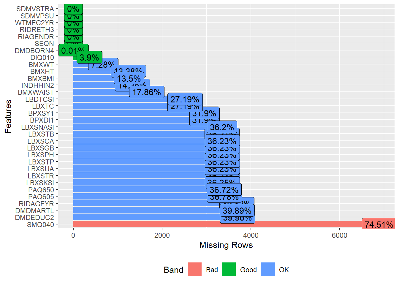
A subsequent chapter will delve into the additional factors that impact how we handle missing data.
Check data summaries
names(analytic.data15)
#>  [1] "SEQN"     "RIAGENDR" "RIDAGEYR" "DMDBORN4" "RIDRETH3" "DMDEDUC2"
#>  [7] "DMDMARTL" "INDHHIN2" "WTMEC2YR" "SDMVPSU"  "SDMVSTRA" "BPXDI1"
#> [13] "BPXSY1"   "BMXWT"    "BMXHT"    "BMXBMI"   "BMXWAIST" "SMQ040"
#> [19] "LBXTC"    "LBDTCSI"  "LBXSTR"   "LBXSUA"   "LBXSTP"   "LBXSTB"
#> [25] "LBXSPH"   "LBXSNASI" "LBXSKSI"  "LBXSGB"   "LBXSCA"   "PAQ605"
#> [31] "PAQ650"   "DIQ010"
names(analytic.data15) <- c("ID", "gender", "age", "born", "race", "education",
"married", "income", "weight", "psu", "strata", "diastolicBP",
"systolicBP", "bodyweight", "bodyheight", "bmi", "waist", "smoke",
"cholesterol", "cholesterolM2", "triglycerides",
"uric.acid", "protein", "bilirubin", "phosphorus", "sodium",
"potassium", "globulin", "calcium", "physical.work",
"physical.recreational","diabetes")
require("tableone")
#> Loading required package: tableone
CreateTableOne(data = analytic.data15, includeNA = TRUE)
#>
#>                                             Overall
#>   n                                             9254
#>   ID (mean (SD))                            98329.50 (2671.54)
#>   gender = Male (%)                             4557 (49.2)
#>   age (mean (SD))                              51.50 (17.81)
#>   born (%)
#>      Born in 50 US states or Washington, DC     7303 (78.9)
#>      Don't know                                    1 ( 0.0)
#>      Others                                     1948 (21.1)
#>      Refused                                       2 ( 0.0)
#>   race (%)
#>      Black                                      2115 (22.9)
#>      Hispanic                                   2187 (23.6)
#>      Other                                      1168 (12.6)
#>      White                                      3150 (34.0)
#>      NA                                          634 ( 6.9)
#>   education (%)
#>      College                                    3114 (33.7)
#>      School                                      479 ( 5.2)
#>      NA                                         5661 (61.2)
#>   married (%)
#>      Married                                    3252 (35.1)
#>      Never.married                              1006 (10.9)
#>      Previously.married                         1305 (14.1)
#>      NA                                         3691 (39.9)
#>   income (%)
#>      <25k                                       1998 (21.6)
#>      Between.25kto54k                           2460 (26.6)
#>      Between.55kto99k                           1843 (19.9)
#>      Over100k                                   1624 (17.5)
#>      NA                                         1329 (14.4)
#>   weight (mean (SD))                        34670.71 (43344.00)
#>   psu (mean (SD))                               1.52 (0.50)
#>   strata (mean (SD))                          140.97 (4.20)
#>   diastolicBP (mean (SD))                      67.84 (16.36)
#>   systolicBP (mean (SD))                      121.33 (19.98)
#>   bodyweight (mean (SD))                       65.14 (32.89)
#>   bodyheight (mean (SD))                      156.59 (22.26)
#>   bmi (mean (SD))                              26.58 (8.26)
#>   waist (mean (SD))                            89.93 (22.81)
#>   smoke (%)
#>      Every.day                                   805 ( 8.7)
#>      Not.at.all                                 1338 (14.5)
#>      Some.days                                   216 ( 2.3)
#>      NA                                         6895 (74.5)
#>   cholesterol (mean (SD))                     179.89 (40.60)
#>   cholesterolM2 (mean (SD))                     4.65 (1.05)
#>   triglycerides (mean (SD))                   137.44 (109.13)
#>   uric.acid (mean (SD))                         5.40 (1.48)
#>   protein (mean (SD))                           7.17 (0.44)
#>   bilirubin (mean (SD))                         0.46 (0.28)
#>   phosphorus (mean (SD))                        3.66 (0.59)
#>   sodium (mean (SD))                          140.32 (2.75)
#>   potassium (mean (SD))                         4.09 (0.36)
#>   globulin (mean (SD))                          3.09 (0.43)
#>   calcium (mean (SD))                           9.32 (0.37)
#>   physical.work (%)
#>      No                                         4461 (48.2)
#>      Yes                                        1389 (15.0)
#>      NA                                         3404 (36.8)
#>   physical.recreational (%)
#>      No                                         4422 (47.8)
#>      Yes                                        1434 (15.5)
#>      NA                                         3398 (36.7)
#>   diabetes (%)
#>      No                                         7816 (84.5)
#>      Yes                                        1077 (11.6)
#>      NA                                          361 ( 3.9)
Create complete case data (for now)
Here cholesterol.bin = 1 denotes desirable cholesterol (< 200 mg/dL), consistent with the 1 = healthy coding used elsewhere in the book. Any logistic regression fit to this variable therefore models the probability of the non-reference level (here, desirable cholesterol), so odds ratios should be read as the odds of desirable cholesterol (e.g., OR < 1 means lower odds of desirable cholesterol).
Creating Table 1 from the complete case data
require("tableone")
CreateTableOne(data = analytic, includeNA = TRUE)
#>
#>                                   Overall
#>   n                                    837
#>   ID (mean (SD))                  98419.74 (2670.63)
#>   gender = Male (%)                    510 (60.9)
#>   age (mean (SD))                    53.44 (16.89)
#>   born = Others (%)                    200 (23.9)
#>   race (%)
#>      Black                             179 (21.4)
#>      Hispanic                          162 (19.4)
#>      Other                              96 (11.5)
#>      White                             400 (47.8)
#>   education = School (%)                94 (11.2)
#>   married (%)
#>      Married                           511 (61.1)
#>      Never.married                     120 (14.3)
#>      Previously.married                206 (24.6)
#>   income (%)
#>      <25k                              215 (25.7)
#>      Between.25kto54k                  256 (30.6)
#>      Between.55kto99k                  202 (24.1)
#>      Over100k                          164 (19.6)
#>   weight (mean (SD))              47722.58 (54356.70)
#>   psu (mean (SD))                     1.46 (0.50)
#>   strata (mean (SD))                141.19 (4.18)
#>   diastolicBP (mean (SD))            71.76 (14.33)
#>   systolicBP (mean (SD))            126.02 (18.12)
#>   bodyweight (mean (SD))             86.48 (22.60)
#>   bodyheight (mean (SD))            169.14 (9.33)
#>   bmi (mean (SD))                    30.16 (7.30)
#>   waist (mean (SD))                 103.32 (17.17)
#>   smoke (%)
#>      Every.day                         228 (27.2)
#>      Not.at.all                        531 (63.4)
#>      Some.days                          78 ( 9.3)
#>   cholesterol (mean (SD))           190.33 (43.16)
#>   cholesterolM2 (mean (SD))           4.92 (1.12)
#>   triglycerides (mean (SD))         156.78 (124.67)
#>   uric.acid (mean (SD))               5.62 (1.46)
#>   protein (mean (SD))                 7.10 (0.42)
#>   bilirubin (mean (SD))               0.46 (0.25)
#>   phosphorus (mean (SD))              3.53 (0.50)
#>   sodium (mean (SD))                140.02 (2.82)
#>   potassium (mean (SD))               4.10 (0.38)
#>   globulin (mean (SD))                3.01 (0.43)
#>   calcium (mean (SD))                 9.31 (0.36)
#>   physical.work = Yes (%)              222 (26.5)
#>   physical.recreational = Yes (%)      203 (24.3)
#>   diabetes = Yes (%)                   179 (21.4)
#>   cholesterol.bin (mean (SD))         0.62 (0.49)
Additional factors come into play when dealing with complex survey datasets; these will be explored in a subsequent chapter.