Chapter 1 Defining Parameter
1.1 Epidemiological research goals
Two common goals for epidemiological research are prediction and causal inference:
- Prediction goal: The primary objective of a prediction goal is to forecast the occurrence or risk of an outcome (\(Y\)) based on one or more risk factors (\(A\)). The focus of this goal is often on making accurate predictions.

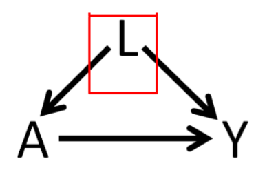
- Causal goal: The causal goal focuses on understanding the causal relationship between a risk factor (often a treatment, \(A\)) and a health outcome (\(Y\)). Control for confounding factors (\(L\)) is often a necessary step in understanding such a relationship. The focus of this goal is often on estimating the parameter ‘treatment effect’.

We only focus on estimating treatment effect today. For that, let us define the notations first.
1.2 Potential outcome
- \(A\): Exposure status
- \(1\) = takes Rosuvastatin
- \(0\) = does not take rosuvastatin
- \(Y\): Outcome: Total cholesterol levels
- \(Y(A=1)\) = potential outcome when exposed
- \(Y(A=0)\) = potential outcome when not exposed
Relationship between \(Y\) and \([Y(A=1), Y(A=0)]\) can be expressed as follows: \(Y = A \times Y(A=1) + (1-A) \times Y(A=0)\)
1.3 Parameters of interest
When assessing the effect of an exposure on an outcome, we are interested about the following estimands
- treatment effect for an individual (TE)
- average treatment effect (ATE)
- average treatment effect on the treated (ATT)
1.3.1 TE
- John takes Rosuvastatin \((A=1)\) and his total cholesterol level is = \(Y(A=1)\) = \(195\) mg/dL (milligrams per deciliter) after 3 months
- John does not take Rosuvastatin \((A=0)\) and his total cholesterol level is = \(Y(A=0)\) = \(245\) mg/dL after 3 months Effect of Rosuvastatin on John is =
\(TE = Y(A=1) - Y(A=0) = 195 - 245 = - 50\)

|
TE is not estimable as we generally can’t observe outcomes under both treatment conditions. |
1.3.2 ATE
Person <- c("John","Jim","Jake","Cody","Luke")
Y1 <- c( 195, 100, 210, 155, 165)
Y0 <- c(245, 160, 270, 210, 230)
PotentialOutcomes <- data.frame(Person, Y1, Y0, TE = Y1-Y0)
mean.values <- c(NA, mean(PotentialOutcomes$Y1),
                 mean(PotentialOutcomes$Y0),
                 mean(PotentialOutcomes$TE))
PotentialOutcomes <- rbind(PotentialOutcomes, mean.values)
kable(PotentialOutcomes, booktabs = TRUE,
             col.names = c("Person", "Y(1)", "Y(0)", "TE")) %>%
row_spec(6, bold = T, color = "white", background = "#D7261E")| Person | Y(1) | Y(0) | TE |
|---|---|---|---|
| John | 195 | 245 | -50 |
| Jim | 100 | 160 | -60 |
| Jake | 210 | 270 | -60 |
| Cody | 155 | 210 | -55 |
| Luke | 165 | 230 | -65 |
| 165 | 223 | -58 |
\(ATE = E[Y(A=1)-Y(A=0)]\)
mean(PotentialOutcomes$Y1 - PotentialOutcomes$Y0)## [1] -581.3.3 Interpretation of ATE
This is a treatment effect (on an average) of the following hypothetical situation
- having the entire population as treated, vs.
- having the entire population as untreated.
Entire population is the reference goup here.
1.3.4 Identifiability Assumptions
Real-world scenario (both outcomes under different treatments can not be observed):
Person <- c("John","Jim","Jake","Cody","Luke")
Y1 <- c( NA, 100, NA, 155, NA)
Y0 <- c(245, NA, 270, NA, 230)
PotentialOutcomes <- data.frame(Person, Y1, Y0, TE = Y1-Y0)
mean.values <- c(NA, mean(PotentialOutcomes$Y1, na.rm = TRUE),
                 mean(PotentialOutcomes$Y0, na.rm = TRUE),
                 mean(PotentialOutcomes$TE))
PotentialOutcomes <- rbind(PotentialOutcomes, round(mean.values,1))
PotentialOutcomes[6,4] <- round(mean(PotentialOutcomes$Y1, na.rm = TRUE)-
                 mean(PotentialOutcomes$Y0, na.rm = TRUE),1)
kable(PotentialOutcomes, booktabs = TRUE,
             col.names = c("Person", "Y(1)", "Y(0)", "TE")) %>%
row_spec(6, bold = T, color = "white", background = "#D7261E")| Person | Y(1) | Y(0) | TE |
|---|---|---|---|
| John | 245.0 | ||
| Jim | 100.0 | ||
| Jake | 270.0 | ||
| Cody | 155.0 | ||
| Luke | 230.0 | ||
| 127.5 | 248.3 | -120.8 |
We can rearrange it as follows:
Person <- c("John","Jim","Jake","Cody","Luke")
A <- c( 0, 1, 0, 1, 0)
Y <- c(245, 100, 270, 155, 230)
RealOutcomes <- data.frame(Person, A, Y)
kable(RealOutcomes, booktabs = TRUE,
col.names = c("Person", "A", "Y")) | Person | A | Y |
|---|---|---|
| John | 0 | 245 |
| Jim | 1 | 100 |
| Jake | 0 | 270 |
| Cody | 1 | 155 |
| Luke | 0 | 230 |
If we can compute a causal quantity, such as \(ATE = E[Y(A=1)-Y(A=0)]\) or mean(PotentialOutcomes$Y1 - PotentialOutcomes$Y0) using a statistical quantity, such as \(E[Y|A=1]-E[Y|A=0]\) or mean(Y[A=1]) - mean(Y[A=0]), we say that the causal quantity is identifiable. For such identifiability, we need to meet the following assumptions:
| Exchangeability | \(Y(1), Y(0) \perp A\) | Treatment assignment is independent of the potential outcome |
| Positivity | \(0 < P(A=1) < 1\) | Subjects are eligible to receive both treatment |
| Consistency | \(Y = Y(a) \forall A=a\) | No multiple version of the treatment |
| No interference | Treated one patient will not impact outcome for others |
Note here, from data we get the estimate of average TE is (100+155)/2 - (245+270+230)/3 = -120.8. Alternatively, we can calculate the beta coefficient associated with \(A\) as follows:
round(coef(lm(Y~A)),1)## (Intercept) A
## 248.3 -120.8Here, beta coefficient associated with \(A\) is -120.8, which is different than average TE -58 that we obtained from the potential outcome data table above. Part of it is because of finite sample bias (having only 5 data points) instead of infinite population. If we had a large enough sample, we would expect the estimate to be close to the true average TE.
You can find more detailed exploration of estimation in a different tutorial using a real data.

Extending these assumptions when confounders exist:
| Conditional Exchangeability | \(Y(1), Y(0) \perp A | L\) | Treatment assignment is independent of the potential outcome, given L |
| Positivity | \(0 < P(A=1 | L) < 1\) | Subjects are eligible to receive both treatment, given L |
Here, - \(L\): Confounder: Age, could be an example
1.3.5 ATT
- Assume that the following are the confounders that impact the relationship between rosuvastatin and cholesterol levels
- race
- sex
- age
- We have 5 Rosuvastatin-treated subjects who are all
- white,
- male,
- 50 years of age
- We recruited additional 5 subjects (same characteristics) to non-rosuvastatin group.
Treated group:
Person <- c("John","Jim","Jake","Cody","Luke")
Y1 <- c( 195, 100, 210, 155, 165)
Y0 <- rep(NA, length(Y1))
Treated <- data.frame(Person, Y1, Y0, TE = Y1-Y0)
Treated[6,2] <- mean(Treated$Y1)
kable(Treated, booktabs = TRUE,
             col.names = c("Person", "Y(1)", "Y(0)", "TE"))%>%
row_spec(6, bold = T, color = "white", background = "#D7261E")| Person | Y(1) | Y(0) | TE |
|---|---|---|---|
| John | 195 | ||
| Jim | 100 | ||
| Jake | 210 | ||
| Cody | 155 | ||
| Luke | 165 | ||
| 165 |
Untreated group: New folks with characteristics similar to the treated group.
Person <- c( "Jack", "Dustin", "Cole", "Lucas", "Dylan")
Y0 <- c( 245, 160, 270, 210, 165)
Y1 <- rep(NA, length(Y0))
Untreated <- data.frame(Person, Y1, Y0, TE = Y1-Y0)
Untreated[6,3] <- mean(Untreated$Y0)
kable(Untreated, booktabs = TRUE,
             col.names = c("Person", "Y(1)", "Y(0)", "TE"))%>%
row_spec(6, bold = T, color = "white", background = "#D7261E")| Person | Y(1) | Y(0) | TE |
|---|---|---|---|
| Jack | 245 | ||
| Dustin | 160 | ||
| Cole | 270 | ||
| Lucas | 210 | ||
| Dylan | 165 | ||
| 210 |
\(ATT = E[Y(A=1)-Y(A=0) | A = 1]\)
mean(Treated$Y1) - mean(Untreated$Y0)## [1] -451.3.6 Interpretation of ATT
This is a treatment effect (on an average) of
- the treated population (reference group), vs.
- untreated population, but have similar characteristics to the reference group/treated population.
It is also possible to change the reference population to untreated population. Then it is called Average Treatment Effect for the Untreated (ATU).