Chapter 2 Balance and Overlap

2.1 Balance

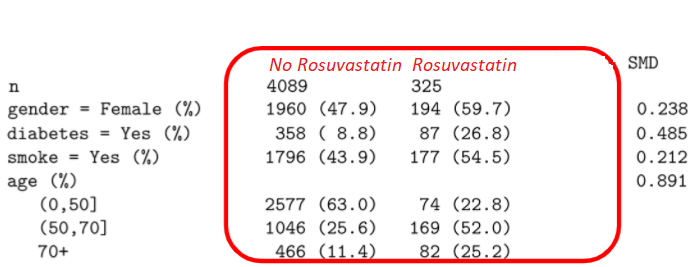
Table 1 in any RCT paper is very important to assess the balance of the baseline characteristics between the two treatment arms.

Balance in RCT:

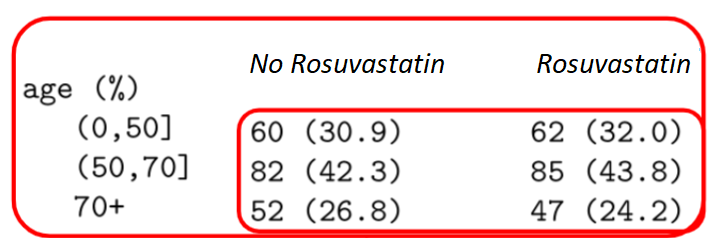Compare the proportions in each age categories by eye-balling in making an evaluation.

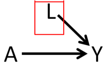
In absence of randomization:

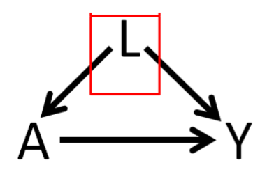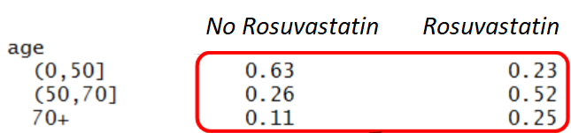2.1.1 Measures of Balance

To compare baseline characteristics between the two treatment groups, we use

t-test (for continuous variables) and
chi-square test (for categorical variables)

Today we will introduce a new concept, known as standardized mean differences (SMD) that can be also used to compare baseline characteristics between the two treatment groups.

2.1.1.1 SMD

Austin (2011b)

For continuous confounders:
- \(SDM_{continuous} = \frac{\bar{L}_{A=1} - \bar{L}_{A=0}}{\sqrt{\frac{(n_1 - 1) \cdot s^2_{A=1} + (n_0 - 1) \cdot s^2_{A=0}}{n_1 + n_0 - 2}}}\)
  - \(\bar{L}_{A=1}\): mean of the continuous variable L for the treated group (A=1)
  - \(\bar{L}_{A=0}\): mean of the continuous variable L for the untreated group (A=0)
  - \(n_1\): number of treated individuals (A=1)
  - \(n_0\): number of untreated individuals (A=0)
  - \(s^2_{A=1}\): variance of the continuous variable L for the treated group (A=1)
  - \(s^2_{A=0}\): variance of the continuous variable L for the untreated group (A=0)
For binary confounders:
- \(SDM_{binary} = \frac{\hat{p}_{A=1} - \hat{p}_{A=0}}{\sqrt{\frac{\hat{p}_{A=1} \times (1 - \hat{p}_{A=1}) + \hat{p}_{A=0} \times (1 - \hat{p}_{A=0})}{2}}}\) where \(\hat{p}{A=1}\) and \(\hat{p}{A=0}\) are the proportions of the two binary groups.
For categorical confounders (more than 2 categories):
- Calculating SMD for categorical variables is slightly more complicated, requiring some additional calculation and averaging out the results from category-specific SMDs. See formulas in Yang and Dalton (2012). It is also possible to report SMD for each category separately (similar to binary).

Generally, \(0.1\) is used as a cut-point. But some suggest more liberal cut-points. More on that later.

COVID example from Gautret et al. (2020)

p-value vs. SMD

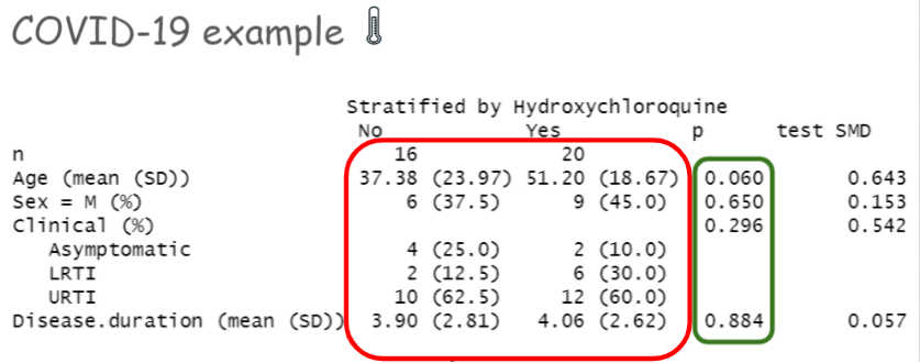
Statistical tests are affected by sample size
- t-test
- McNemar tests
- Wilcoxon rank test
Balance of what?
- statistical tests make inference about balance at the population level
- but we are really interested in balance at the sample level

2.1.1.2 Variance ratio

Variances of baseline characteristics between comparator groups under consideration. Suggested cut-point rages are (0.5 to 2). More liberal cut-points are also used in the literature. More on this later.

2.2 Adjustment

2.2.1 Why adjust?

In absence of randomization, treatment effect estimate ATE = \(E[Y|A=1] - E[Y|A=0]\) includes

Treatment effect
Systematic differences in 2 groups (‘confounding’)
- Doctors may prescribe tx more to frail and older age patients.
- In here, \(L\) = age is a confounder.

In absence of randomization, if age is a known confounder, conditioning can solve the problem:

Causal effect for young (\(<50\))	\(E[Y\|A=1, L =\) `younger age`\(]\) - \(E[Y\|A=0, L =\) `younger age`\(]\)
Causal effect for old (\(\ge 50\))	\(E[Y\|A=1, L =\) `older age`\(]\) - \(E[Y\|A=0, L =\) `older age`\(]\)

Conditional exchangeability; only works if \(L\) is measured.

2.2.2 Adjustment Methods

Adjustment of imbalance could mean

exact matching (Rubin 1973)
stratification, restriction

When L includes a large number of covariates, matching method would result in a small sample size.

Regression and machine learning methods are popular adjustment methods. Below is a list of adjustment methods that uses different combinations of exposure and outcome modelling.

Method	Exposure model \((\color{green}{\text{A}} \sim ...)\)	Outcome Model \((Y \sim ...)\)
Regression (Gauss 1821 \(\dagger\))	No \(\color{green}{\text{A}}\) modelling	Yes \((Y \sim \color{green}{\text{A}}+\color{red}{\text{L}})\)
Instrumental variable methods (2SLS) \(\dagger\dagger\)	\(A \sim IV + L\), but explicitly to obtain \(\hat{A}\)	\(Y \sim \hat{A} + L\)
Propensity score matching (Rosenbaum and Rubin 1983)	Yes \((\color{green}{\text{A}} \sim \color{red}{\text{L}})\)	Crude comparison on matched data \((Y \sim \color{green}{\text{A}})\)
Propensity score Weighting (Rosenbaum and Rubin 1983)	Yes \((\color{green}{\text{A}} \sim \color{red}{\text{L}})\)	Crude comparison on weighted data \((Y \sim \color{green}{\text{A}})\)
Propensity score double adjustment	Yes \((\color{green}{\text{A}} \sim \color{red}{\text{L}})\)	Yes \((Y \sim \color{green}{\text{A}}+ \color{red}{\text{L}})\)
Decision tree-based method (Breiman et al. 1984)	No \(\color{green}{\text{A}}\) modelling	Yes \((Y \sim \color{green}{\text{A}}+\color{red}{\text{L}})\)
G-Computation (J. Robins 1986)	No \(\color{green}{\text{A}}\) modelling	Yes \((Y \sim \color{green}{\text{A=1 vs. 0}}+\color{red}{\text{L}})\)
Random Forest (Ho 1995)	No \(\color{green}{\text{A}}\) modelling	Yes \((Y \sim \color{green}{\text{A}}+\color{red}{\text{L}})\)
Double robust (J. M. Robins and Rotnitzky 2001), (Van Der Laan and Rubin 2006) (augmented weighted, or TMLE), causal forest (Athey and Wager 2019), double machine learning (DML) (Chernozhukov et al. 2017), potentially using machine learning	Yes \((\color{green}{\text{A}} \sim \color{red}{\text{L}})\)	Yes \((Y \sim \color{green}{\text{A}}+ \color{red}{\text{L}})\)

\(\dagger\) (Stanton 2001). \(\dagger\dagger\) other economic models also exists: Structural equation modeling, Difference-in-differences, Regression discontinuity, Interrupted time series

2.3 Lack of overlap

“Lack of complete overlap” happens if there is a baseline covariate space where there are exposed patients, but no control or vice versa.
- Region of ‘no overlap’ is an inherent limitation of the data.

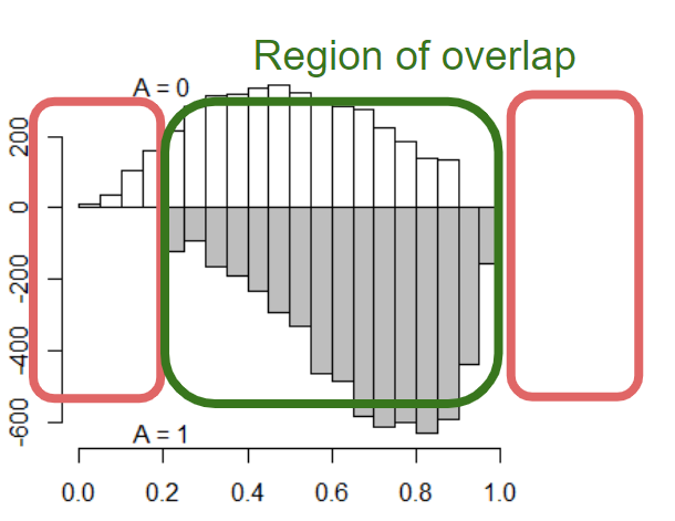
Regression adjustment usually do not offer any solution to this.
- Consequently, inference is not generalizable beyond the region of overlap.

References

Athey, Susan, and Stefan Wager. 2019. “Estimating Treatment Effects with Causal Forests: An Application.” Observational Studies 5 (2): 37–51.

———. 2011b. “An Introduction to Propensity Score Methods for Reducing the Effects of Confounding in Observational Studies.” Multivariate Behavioral Research 46 (3): 399–424.

Breiman, L, JH Friedman, R Olshen, and CJ Stone. 1984. “Classification and Regression Trees.”

Chernozhukov, Victor, Denis Chetverikov, Mert Demirer, Esther Duflo, Christian Hansen, and Whitney Newey. 2017. “Double/Debiased/Neyman Machine Learning of Treatment Effects.” American Economic Review 107 (5): 261–65.

Gautret, Philippe, Jean-Christophe Lagier, Philippe Parola, Line Meddeb, Morgane Mailhe, Barbara Doudier, Johan Courjon, et al. 2020. “Hydroxychloroquine and Azithromycin as a Treatment of COVID-19: Results of an Open-Label Non-Randomized Clinical Trial.” International Journal of Antimicrobial Agents 56 (1): 105949.

Ho, Tin Kam. 1995. “Random Decision Forests.” In Proceedings of 3rd International Conference on Document Analysis and Recognition, 1:278–82. IEEE.

Robins, J. M., and A G Rotnitzky. 2001. “Comment on the Bickel and Kwon Article, ’Inference for Semiparametric Models: Some Questions and an Answer’.” Statistica Sinica 11 (January): 920–36.

Robins, James. 1986. “A New Approach to Causal Inference in Mortality Studies with a Sustained Exposure Period—Application to Control of the Healthy Worker Survivor Effect.” Mathematical Modelling 7 (9-12): 1393–1512.

Rosenbaum, Paul R, and Donald B Rubin. 1983. “The Central Role of the Propensity Score in Observational Studies for Causal Effects.” Biometrika 70 (1): 41–55.

Rubin, Donald B. 1973. “Matching to Remove Bias in Observational Studies.” Biometrics, 159–83.

Stanton, Jeffrey M. 2001. “Galton, Pearson, and the Peas: A Brief History of Linear Regression for Statistics Instructors.” Journal of Statistics Education 9 (3).

Van Der Laan, Mark J, and Daniel Rubin. 2006. “Targeted Maximum Likelihood Learning.” The International Journal of Biostatistics 2 (1).

Yang, Dongsheng, and Jarrod E Dalton. 2012. “A Unified Approach to Measuring the Effect Size Between Two Groups Using SAS.” In SAS Global Forum, 335:1–6. Citeseer.