Chapter 2 G-computation
2.1 Closer look at the data
# Read the data saved at the last chapter
ObsData <- readRDS(file = "data/rhcAnalytic.RDS")
dim(ObsData)
## [1] 5735 51In this dataset, we have
- 5,735 subjects,
- 1 outcome variable (\(Y\) = length of stay),
- 1 exposure variable (\(A\) = RHC status), and
- 49 covariates.
2.1.1 View data from 6 participants
small.data <- ObsData[1:6,c("sex","A","Y")]
kable(small.data)| sex | A | Y |
|---|---|---|
| Male | 0 | 9 |
| Female | 1 | 45 |
| Female | 1 | 60 |
| Female | 0 | 37 |
| Male | 1 | 2 |
| Female | 0 | 7 |
2.1.2 New notations
| Notations | Example in RHC study |
|---|---|
| \(A\): Exposure status | RHC |
| \(Y\): Observed outcome | length of stay |
| \(Y(A=1)\) = potential outcome when exposed | length of stay when RHC used |
| \(Y(A=0)\) = potential outcome when not exposed | length of stay when RHC not used |
| \(L\): covariates | \(49\) covariates |
For explaining the concepts in this chapter, we will convert our data representation
- from
| Covariate | Exposure | Observed outcome |
|---|---|---|
| \(L\) | \(A\) | \(Y\) |
| sex | RHC |
length of stay |
- to the following representation:
| Covariate | Exposure | Outcome under exposed | Outcome under unexposed |
|---|---|---|---|
| \(L\) | \(A\) | \(Y(A=1)\) | \(Y(A=0)\) |
| sex | RHC |
length of stay under RHC |
length of stay under no RHC |
2.1.3 Restructure the data to estimate treatment effect
In causal inference literature, often the data is structured in such a way that the outcomes \(Y\) under different treatments \(A\) are in different columns. What we are doing here is we are distinguishing \(Y(A=1)\) from \(Y(A=0)\).
small.data$id <- c("John","Emma","Isabella","Sophia","Luke", "Mia")
small.data$Y1 <- ifelse(small.data$A==1, small.data$Y, NA)
small.data$Y0 <- ifelse(small.data$A==0, small.data$Y, NA)
small.data$TE <- small.data$Y1 - small.data$Y0
small.data <- small.data[c("id", "sex","A","Y1","Y0", "TE")]
small.data$Y <- NULL
small.data$sex <- as.character(small.data$sex)
m.Y1 <- mean(small.data$Y1, na.rm = TRUE)
m.Y0 <- mean(small.data$Y0, na.rm = TRUE)
mean.values <- round(c(NA,NA, NA, m.Y1, m.Y0,
                 m.Y1 - m.Y0),0)
small.data2 <- rbind(small.data, mean.values)
kable(small.data2, booktabs = TRUE, digits=1,
             col.names = c("Subject ID","Sex",
                           "RHC status (A)",
                           "Y when A=1 (RHC)",
                           "Y when A=0 (no RHC)",
                           "Treatment Effect"))%>%
  row_spec(7, bold = TRUE, color = "white",
background = "#D7261E")| Subject ID | Sex | RHC status (A) | Y when A=1 (RHC) | Y when A=0 (no RHC) | Treatment Effect |
|---|---|---|---|---|---|
| John | Male | 0 | 9 | ||
| Emma | Female | 1 | 45 | ||
| Isabella | Female | 1 | 60 | ||
| Sophia | Female | 0 | 37 | ||
| Luke | Male | 1 | 2 | ||
| Mia | Female | 0 | 7 | ||
| 36 | 18 | 18 |
Then it is easy to see
- the mean outcome under treated group (
RHC) - the mean outcome under untreated group (
no RHC)
and the difference between these two means is the treatment effect.
2.1.4 Treat the problem as a missing value problem
Restructure the problem as a missing data problem.
Instead of just estimating treatment effect on an average level, an alternate could be to
- impute mean outcomes for the treated subjects
- impute mean outcomes for the untreated subjects
- Calculate individual treatment effect estimate
- then calculate the average treatment effect
small.data0 <- small.data
small.data$Y1[is.na(small.data$Y1)] <- round(m.Y1)
small.data$Y0[is.na(small.data$Y0)] <- round(m.Y0)
small.data$TE <- small.data$Y1 - small.data$Y0
m.Y1 <- mean(small.data$Y1)
m.Y1
## [1] 35.83333m.Y0 <- mean(small.data$Y0)
m.Y0## [1] 17.83333m.TE <- mean(small.data$TE)
mean.values <- round(c(NA,NA, NA, m.Y1, m.Y0, m.TE),0)
small.data2 <- rbind(small.data, mean.values)
small.data2$Y1[1:6] <- cell_spec(small.data2$Y1[1:6],
color = ifelse(small.data2$Y1[1:6]
== round(m.Y1),
"red", "black"),
background = ifelse(small.data2$Y1[1:6]
== round(m.Y1),
"yellow", "white"),
bold = ifelse(small.data2$Y1[1:6]
== round(m.Y1),
TRUE, FALSE))
small.data2$Y0[1:6] <- cell_spec(small.data2$Y0[1:6],
color = ifelse(small.data2$Y0[1:6]
== round(m.Y0),
"red", "black"),
background = ifelse(small.data2$Y0[1:6]
== round(m.Y0),
"yellow", "white"),
bold = ifelse(small.data2$Y0[1:6]
== round(m.Y0),
TRUE, FALSE))
kable(small.data2, booktabs = TRUE,
digits=1, escape = FALSE,
col.names = c("Subject ID","Sex",
"RHC status (A)",
"Y when A=1 (RHC)",
"Y when A=0 (no RHC)",
"Treatment Effect"))%>%
row_spec(7, bold = TRUE, color = "white",
background = "#D7261E")| Subject ID | Sex | RHC status (A) | Y when A=1 (RHC) | Y when A=0 (no RHC) | Treatment Effect |
|---|---|---|---|---|---|
| John | Male | 0 | 36 | 9 | 27 |
| Emma | Female | 1 | 45 | 18 | 27 |
| Isabella | Female | 1 | 60 | 18 | 42 |
| Sophia | Female | 0 | 36 | 37 | -1 |
| Luke | Male | 1 | 2 | 18 | -16 |
| Mia | Female | 0 | 36 | 7 | 29 |
| 36 | 18 | 18 |
2.1.5 Impute better value?
Assume that sex variable is acting as a confounder. Then, it might make more sense to restrict imputing outcome values specific to male and female participants.
- impute means specific to males for male subjects, and separately
- impute means specific to females for female subjects.
small.data <- small.data0
m.Y1m <- mean(small.data$Y1[small.data$sex == "Male"], na.rm = TRUE)
m.Y1m
## [1] 2m.Y1f <- mean(small.data$Y1[small.data$sex == "Female"], na.rm = TRUE)
m.Y1f## [1] 52.5m.Y0m <- mean(small.data$Y0[small.data$sex == "Male"], na.rm = TRUE)
m.Y0m## [1] 9m.Y0f <- mean(small.data$Y0[small.data$sex == "Female"], na.rm = TRUE)
m.Y0f## [1] 22m.TE.m <- m.Y1m-m.Y0m
m.TE.f <- m.Y1f-m.Y0f
mean.values.m <- c(NA,"Mean for males", NA, round(c(m.Y1m, m.Y0m, m.TE.m),1))
mean.values.f <- c(NA,"Mean for females", NA, round(c(m.Y1f, m.Y0f, m.TE.f),1))
small.data$Y1[small.data$sex ==
"Male"][is.na(small.data$Y1[small.data$sex ==
"Male"])] <- round(m.Y1m,1)
small.data$Y0[small.data$sex ==
"Male"][is.na(small.data$Y0[small.data$sex ==
"Male"])] <- round(m.Y0m,1)
small.data$Y1[small.data$sex ==
"Female"][is.na(small.data$Y1[small.data$sex ==
"Female"])] <- round(m.Y1f,1)
small.data$Y0[small.data$sex ==
"Female"][is.na(small.data$Y0[small.data$sex ==
"Female"])] <- round(m.Y0f,1)
small.data$TE <- small.data$Y1 - small.data$Y0
small.data2 <- rbind(small.data, mean.values.m,mean.values.f)
small.data2$Y1[1] <- cell_spec(round(m.Y1m,1), bold = TRUE,
color = "red", background = "yellow")
small.data2$Y0[5] <- cell_spec(round(m.Y0m,1), bold = TRUE,
color = "red", background = "yellow")
small.data2$Y1[c(4,6)] <- cell_spec(round(m.Y1f,1), bold = TRUE,
color = "blue", background = "yellow")
small.data2$Y0[c(2,3)] <- cell_spec(round(m.Y0f,1), bold = TRUE,
color = "blue", background = "yellow")
kable(small.data2, booktabs = TRUE,
digits=1, escape = FALSE,
col.names = c("Subject ID","Sex","RHC status (A)",
"Y when A=1 (RHC)", "Y when A=0 (no RHC)",
"Treatment Effect"))%>%
row_spec(7, bold = TRUE, color = "white", background = "red")%>%
row_spec(8, bold = TRUE, color = "white", background = "blue")| Subject ID | Sex | RHC status (A) | Y when A=1 (RHC) | Y when A=0 (no RHC) | Treatment Effect |
|---|---|---|---|---|---|
| John | Male | 0 | 2 | 9 | -7 |
| Emma | Female | 1 | 45 | 22 | 23 |
| Isabella | Female | 1 | 60 | 22 | 38 |
| Sophia | Female | 0 | 52.5 | 37 | 15.5 |
| Luke | Male | 1 | 2 | 9 | -7 |
| Mia | Female | 0 | 52.5 | 7 | 45.5 |
| Mean for males | 2 | 9 | -7 | ||
| Mean for females | 52.5 | 22 | 30.5 |
- Extending the problem to other covariates, you can see that we could condition on rest of the covariates (such as age, income, race, disease category) to get better imputation values.
Regression is a generalized method to take mean conditional on many covariates.
2.2 Use Regression for predicting outcome
Let us fit the outcome with all covariates, including the exposure status.
# isolate the names of baseline covariates
baselinevars <- names(dplyr::select(ObsData, !c(A,Y)))
# adjust the exposure variable (primary interest) + covariates
out.formula <- as.formula(paste("Y~ A +",
                               paste(baselinevars,
                                     collapse = "+")))
fit1 <- lm(out.formula, data = ObsData)
coef(fit1)
## (Intercept) A
## -7.680847e+01 2.902030e+00
## Disease.categoryCHF Disease.categoryOther
## -5.594331e+00 -4.421893e+00
## Disease.categoryMOSF CancerLocalized (Yes)
## 2.873451e+00 -7.794459e+00
## CancerMetastatic Cardiovascular1
## -1.056549e+01 6.605038e-01
## Congestive.HF1 Dementia1
## -1.754818e+00 -1.261136e+00
## Psychiatric1 Pulmonary1
## -4.841489e-01 2.063282e+00
## Renal1 Hepatic1
## -6.935923e+00 -1.523238e+00
## GI.Bleed1 Tumor1
## -5.096253e+00 4.573818e+00
## Immunosupperssion1 Transfer.hx1
## 1.103694e-01 1.161342e+00
## MI1 age[50,60)
## -1.650935e+00 1.429833e-01
## age[60,70) age[70,80)
## -4.055267e-01 -1.103439e+00
## age[80, Inf) sexFemale
## -2.757278e+00 8.272236e-01
## edu DASIndex
## 4.775891e-02 -5.343588e-02
## APACHE.score Glasgow.Coma.Score
## -7.020692e-02 1.563055e-02
## blood.pressure WBC
## -1.323182e-02 3.940879e-02
## Heart.rate Respiratory.rate
## 2.244431e-02 -1.467861e-03
## Temperature PaO2vs.FIO2
## 5.086475e-01 -8.517735e-03
## Albumin Hematocrit
## -2.570965e+00 -1.951544e-01
## Bilirubin Creatinine
## -9.814574e-02 5.210509e-01
## Sodium Potassium
## 1.365534e-01 3.447162e-01
## PaCo2 PH
## 1.165866e-01 1.005261e+01
## Weight DNR.statusYes
## 2.257116e-04 -7.959037e+00
## Medical.insuranceMedicare Medical.insuranceMedicare & Medicaid
## -5.174593e-01 -2.422199e+00
## Medical.insuranceNo insurance Medical.insurancePrivate
## -1.785085e+00 -2.086480e+00
## Medical.insurancePrivate & Medicare Respiratory.DiagYes
## -2.018369e+00 3.404743e-01
## Cardiovascular.DiagYes Neurological.DiagYes
## 3.784972e-01 3.541516e+00
## Gastrointestinal.DiagYes Renal.DiagYes
## 2.551541e+00 1.784893e+00
## Metabolic.DiagYes Hematologic.DiagYes
## -1.161415e+00 -3.858024e+00
## Sepsis.DiagYes Trauma.DiagYes
## 2.716148e-03 1.112049e+00
## Orthopedic.DiagYes raceblack
## 3.543464e+00 -1.149936e+00
## raceother income$25-$50k
## 2.467487e-01 2.459547e+00
## income> $50k incomeUnder $11k
## 4.214815e-01 -4.284414e-012.2.1 Predict outcome for treated
- Using the regression fit, we can obtain predicted outcome values for the treated.
- We are not only predicting for the unobserved, but also for the observed values when a person was treated.
ObsData$Pred.Y1 <- predict(fit1,
                           newdata = data.frame(A = 1,
                                                dplyr::select(ObsData, !A)),
                           type = "response")
Mean predicted outcome for treated
mean(ObsData$Pred.Y1)## [1] 23.35625hist(ObsData$Pred.Y1,
main = "Histogram for predicted outcome for treated",
xlab = "Y(A=1)")
abline(v=mean(ObsData$Pred.Y1),col="blue", lwd = 4)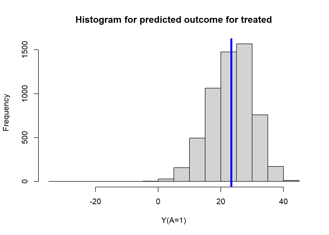
2.2.2 Look at the predicted outcome data for treated
small.data1 <- ObsData[1:6,c("A","Pred.Y1")]
small.data1$id <- c("John","Emma","Isabella","Sophia","Luke", "Mia")
small.data1 <- small.data1[c("id", "A","Pred.Y1")]
kable(small.data1, booktabs = TRUE, digits=1,
             col.names = c("id","RHC status (A)",
"Y.hat when A=1 (RHC)"))| id | RHC status (A) | Y.hat when A=1 (RHC) |
|---|---|---|
| John | 0 | 17.5 |
| Emma | 1 | 28.7 |
| Isabella | 1 | 24.6 |
| Sophia | 0 | 21.6 |
| Luke | 1 | 13.6 |
| Mia | 0 | 25.5 |
2.2.3 Predict outcome for untreated
ObsData$Pred.Y0 <- predict(fit1,
                           newdata = data.frame(A = 0,
                                                dplyr::select(ObsData, !A)),
                           type = "response")
Mean predicted outcome for untreated
mean(ObsData$Pred.Y0)## [1] 20.45422hist(ObsData$Pred.Y0,
main = "Histogram for predicted outcome for untreated",
xlab = "Y(A=0)")
abline(v=mean(ObsData$Pred.Y0),col="blue", lwd = 4)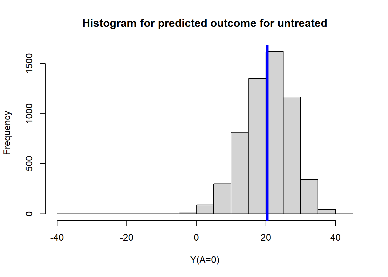
2.2.4 Look at the predicted outcome data for untreated
small.data0 <- ObsData[1:6,c("A","Pred.Y0")]
small.data0$id <- c("John","Emma","Isabella","Sophia","Luke", "Mia")
small.data0 <- small.data0[c("id", "A","Pred.Y0")]
kable(small.data0, booktabs = TRUE, digits=1,
             col.names = c("id","RHC status (A)",
"Y.hat when A=0 (no RHC)"))| id | RHC status (A) | Y.hat when A=0 (no RHC) |
|---|---|---|
| John | 0 | 14.6 |
| Emma | 1 | 25.8 |
| Isabella | 1 | 21.7 |
| Sophia | 0 | 18.7 |
| Luke | 1 | 10.7 |
| Mia | 0 | 22.6 |
2.2.5 Look at the predicted outcome data for all!
small.data01 <- small.data1
small.data01$Pred.Y0 <- small.data0$Pred.Y0
small.data01$Pred.TE <- small.data01$Pred.Y1 - small.data01$Pred.Y0
m.Y1 <- mean(small.data01$Pred.Y1)
m.Y0 <- mean(small.data01$Pred.Y0)
mean.values <- round(c(NA,NA, m.Y1, m.Y0, m.Y1 -m.Y0),1)
small.data2 <- rbind(small.data01, mean.values)
kable(small.data2, booktabs = TRUE, digits=1,
             col.names = c("id","RHC status (A)",
                           "Y.hat when A=1 (RHC)",
                           "Y.hat when A=0 (no RHC)",
                           "Treatment Effect"))%>%
row_spec(7, bold = TRUE, color = "white", background = "#D7261E")| id | RHC status (A) | Y.hat when A=1 (RHC) | Y.hat when A=0 (no RHC) | Treatment Effect |
|---|---|---|---|---|
| John | 0 | 17.5 | 14.6 | 2.9 |
| Emma | 1 | 28.7 | 25.8 | 2.9 |
| Isabella | 1 | 24.6 | 21.7 | 2.9 |
| Sophia | 0 | 21.6 | 18.7 | 2.9 |
| Luke | 1 | 13.6 | 10.7 | 2.9 |
| Mia | 0 | 25.5 | 22.6 | 2.9 |
| 21.9 | 19.0 | 2.9 |
From this table, it is easy to calculate treatment effect estimate.
The process we just went through, is a version of parametric G-computation!
2.3 Parametric G-computation
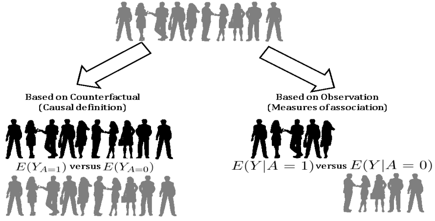
Figure 2.1: Defining treatment effect in terms of potential outcomes and observations
2.3.1 Steps
| Step 1 | Fit the outcome regression on the exposure and covariates: \(Y \sim A + L\) |
| Step 2 | Extract outcome prediction for treated \(\hat{Y}_{A=1}\) by setting all \(A=1\) |
| Step 3 | Extract outcome prediction for untreated \(\hat{Y}_{A=0}\) by setting all \(A=0\) |
| Step 4 | Subtract the mean of these two outcome predictions to get treatment effect estimate: \(TE = E(\hat{Y}_{A=1}) - E(\hat{Y}_{A=0})\) |
2.3.1.1 Step 1
Fit the outcome regression on the exposure and covariates: \(Y \sim A + L\)
out.formula <- as.formula(paste("Y~ A +",
                               paste(baselinevars,
                                     collapse = "+")))
fit1 <- lm(out.formula, data = ObsData)
\(Q(A,L)\) is often used to represent the predictions from the G-comp model.
2.3.1.2 Step 2
Extract outcome prediction for treated \(\hat{Y}_{A=1}\) by setting all \(A=1\)|
ObsData$Pred.Y1 <- predict(fit1,
                           newdata = data.frame(A = 1,
                                                dplyr::select(ObsData, !A)),
                           type = "response")
2.3.1.3 Step 3
Extract outcome prediction for untreated \(\hat{Y}_{A=0}\) by setting all \(A=0\)
ObsData$Pred.Y0 <- predict(fit1,
                           newdata = data.frame(A = 0,
                                                dplyr::select(ObsData, !A)),
                           type = "response")
2.3.1.4 Step 4
Subtract the mean of these two outcome predictions to get treatment effect estimate: \(TE = E(\hat{Y}_{A=1}) - E(\hat{Y}_{A=0})\)
ObsData$Pred.TE <- ObsData$Pred.Y1 - ObsData$Pred.Y0 2.3.2 Treatment effect estimate
Mean value of predicted treatment effect
TE <- mean(ObsData$Pred.TE)
TE
## [1] 2.90203SD of treatment effect
sd(ObsData$Pred.TE)## [1] 5.132733e-15hist(ObsData$Pred.TE,
main = "Histogram for predicted treatment effect",
xlab = "Y(A=1) - Y(A=0)")## Warning in plot.window(xlim, ylim, "", ...): relative range of values ( 93 *
## EPS) is small (axis 1)abline(v=mean(ObsData$Pred.TE),col="blue", lwd = 4)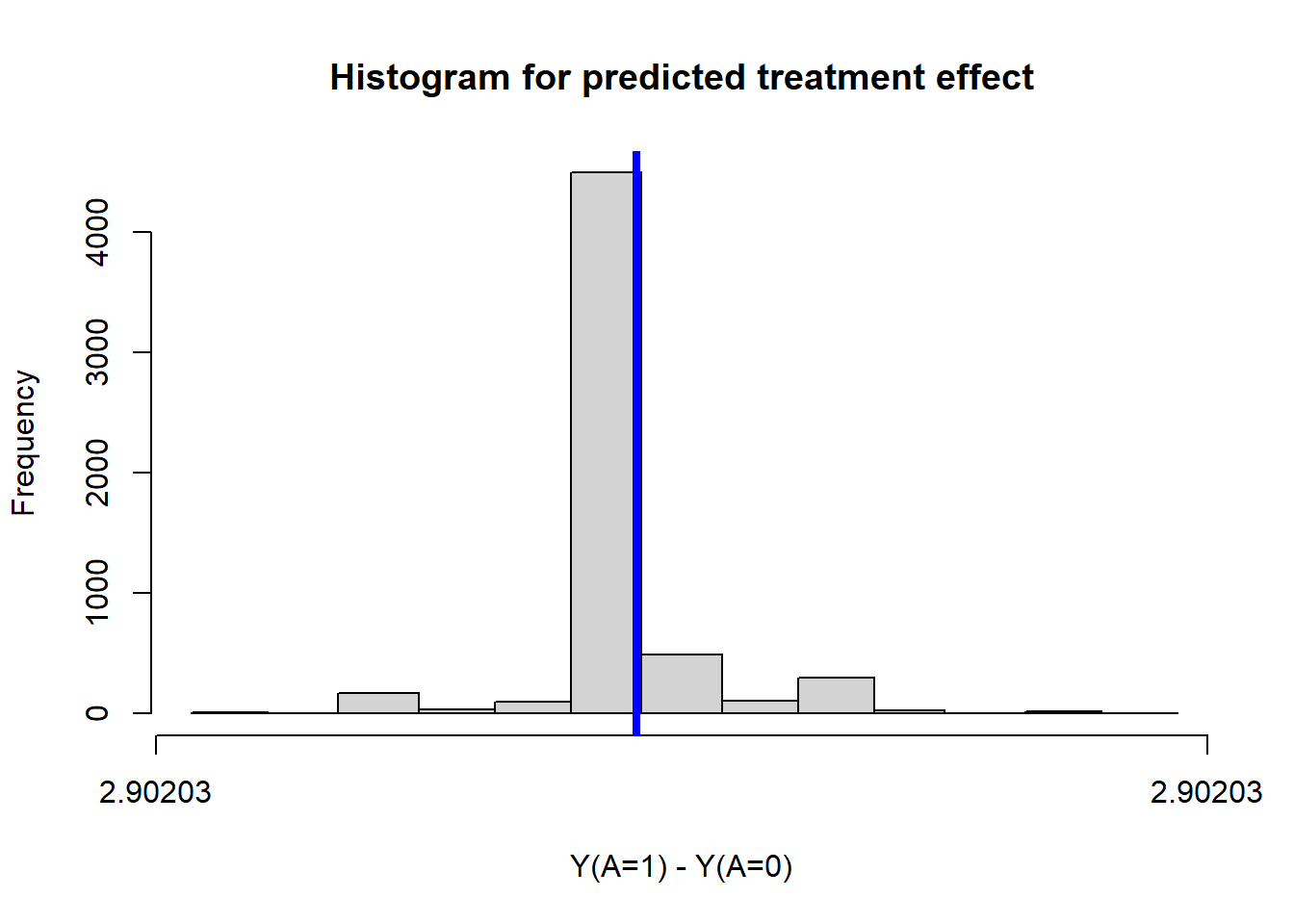
This shows that the SD estimate is useless from g-computation method directly.
2.4 Estimating the confidence intervals
We already have an idea about the point estimate of the treatment effect:
mean(ObsData$Pred.TE)## [1] 2.90203For confidence interval estimates for G-computation, bootstrap would be necessary.
In the following example, we use \(R = 250\).
require(boot)
gcomp.boot <- function(formula = out.formula, data = ObsData, indices) {
  boot_sample <- data[indices, ]
  fit.boot <- lm(formula, data = boot_sample)
  Pred.Y1 <- predict(fit.boot,
                     newdata = data.frame(A = 1,
                                          dplyr::select(boot_sample, !A)),
                           type = "response")
  Pred.Y0 <- predict(fit.boot,
                     newdata = data.frame(A = 0,
                                          dplyr::select(boot_sample, !A)),
                           type = "response")
  Pred.TE <- mean(Pred.Y1) - mean(Pred.Y0)
  return(Pred.TE)
}
set.seed(123)
gcomp.res <- boot(data=ObsData,
                  statistic=gcomp.boot,
                  R=250,
                  formula=out.formula)
Below we show the resulting estimates from \(R\) bootstrap samples.
plot(gcomp.res) 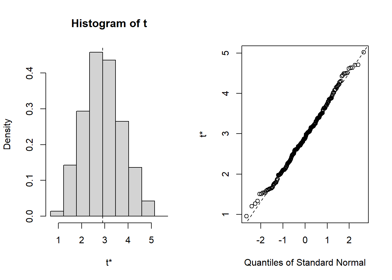
Below are two versions of confidence interval.
- One is based on normality assumption: point estimate - and + with 1.96 multiplied by SD estimate
- Another is based on percentiles
CI1 <- boot.ci(gcomp.res, type="norm")
CI1
## BOOTSTRAP CONFIDENCE INTERVAL CALCULATIONS
## Based on 250 bootstrap replicates
##
## CALL :
## boot.ci(boot.out = gcomp.res, type = "norm")
##
## Intervals :
## Level Normal
## 95% ( 1.315, 4.444 )
## Calculations and Intervals on Original ScaleCI2 <- boot.ci(gcomp.res, type="perc")
CI2## BOOTSTRAP CONFIDENCE INTERVAL CALCULATIONS
## Based on 250 bootstrap replicates
##
## CALL :
## boot.ci(boot.out = gcomp.res, type = "perc")
##
## Intervals :
## Level Percentile
## 95% ( 1.515, 4.589 )
## Calculations and Intervals on Original Scale
## Some percentile intervals may be unstablesaveRDS(TE, file = "data/gcomp.RDS")
saveRDS(CI2, file = "data/gcompci.RDS")
Let’s focus on only first 6 columns, with only 3 variables.