Chapter 8 PS vs. Regression
8.1 Data Simulation
Simplified simulation example, so that we know the true parameter \(\theta\).
| \(Y\) : Outcome | Cholesterol levels (continuous) |
| \(A\) : Exposure | Diabetes |
| \(L\) : Known Confounders | age (continuous) |
- Confounder \(L\) (continuous)
- \(L\) ~ N(mean = 10, sd = 1)
- Treatment \(A\) (binary 0/1)
- Logit \(P(A = 1)\) ~ 0.4 L
- Outcome \(Y\) (continuous)
- Y ~ N(mean = 3 L + \(\theta\) A, sd = 1)
True parameter: \(\theta = 0.7\)
- We want to see, how close the estimates (compared to this \(\theta = 0.7\)) are when we try to estimate this parameter using different methods:
- regression
- PS
Note that, given the data generating mechanism, \(L\) is a confounders, and should be adjusted.
require(simcausal)
D <- DAG.empty()
D <- D +
  node("L", distr = "rnorm", mean = 10, sd = 1) +
  node("A", distr = "rbern", prob = plogis(0.4*L)) +
  node("Y", distr = "rnorm", mean = 3 * L + 0.7 * A, sd = 1)
Dset <- set.DAG(D)plotDAG(Dset, xjitter = 0.1, yjitter = .9,
edge_attrs = list(width = 0.5, arrow.width = 0.4, arrow.size = 1.7),
vertex_attrs = list(size = 18, label.cex = 1.8))## using the following vertex attributes:## 181.8NAdarkbluenone0## using the following edge attributes:## 0.50.41.7black1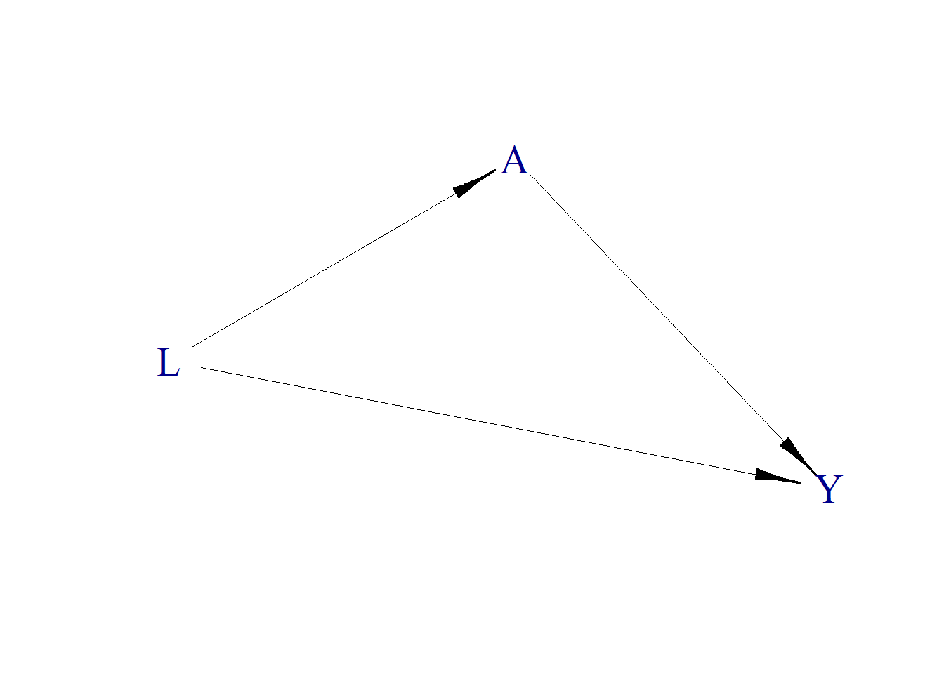
# Data generating function
fnc <- function(n = 10, seedx = 123){
  require(simcausal)
  set.seed(seedx)
  D <- DAG.empty()
  D <- D +
    node("L", distr = "rnorm", mean = 10, sd = 1) +
    node("A", distr = "rbern", prob = plogis(0.4*L)) +
    node("Y", distr = "rnorm", mean = 3 * L + 0.7 * A, sd = 1)
  Dset <- set.DAG(D)
  A1 <- node("A", distr = "rbern", prob = 1)
  Dset <- Dset + action("A1", nodes = A1)
  A0 <- node("A", distr = "rbern", prob = 0)
  Dset <- Dset + action("A0", nodes = A0)
  Cdat <- sim(DAG = Dset, actions = c("A1", "A0"), n = n, rndseed = 123)
  generated.data <- round(cbind(Cdat$A1[c("ID", "L", "Y")],Cdat$A0[c("Y")]),2)
  names(generated.data) <- c("ID", "L", "Y1", "Y0")
  generated.data <- generated.data[order(generated.data$L, generated.data$ID),]
  generated.data$A <- sample(c(0,1),n, replace = TRUE)
  generated.data$Y <- ifelse(generated.data$A==0, generated.data$Y0, generated.data$Y1)
  counterfactual.dataset<- generated.data[order(generated.data$ID) , ][c("ID","L","A","Y1","Y0")]
  observed.dataset<- generated.data[order(generated.data$ID) , ][c("ID","L","A","Y")]
  return(list(counterfactual=counterfactual.dataset,
              observed=observed.dataset))
}
10 observations from the data generation:
result.data <- fnc(n=10) result.data## $counterfactual
## ID L A Y1 Y0
## 1 1 9.44 0 30.24 29.54
## 2 2 9.77 1 30.37 29.67
## 3 3 11.56 0 35.78 35.08
## 4 4 10.07 0 31.02 30.32
## 5 5 10.13 1 30.53 29.83
## 6 6 11.72 0 37.63 36.93
## 7 7 10.46 1 32.58 31.88
## 8 8 8.73 0 24.94 24.24
## 9 9 9.31 0 29.34 28.64
## 10 10 9.55 1 28.89 28.19
##
## $observed
## ID L A Y
## 1 1 9.44 0 29.54
## 2 2 9.77 1 30.37
## 3 3 11.56 0 35.08
## 4 4 10.07 0 30.32
## 5 5 10.13 1 30.53
## 6 6 11.72 0 36.93
## 7 7 10.46 1 32.58
## 8 8 8.73 0 24.24
## 9 9 9.31 0 28.64
## 10 10 9.55 1 28.898.2 Treatment effect from counterfactuals
True \(\theta\) can be obtained from counterfactual data:
result.data$counterfactual$TE <- result.data$counterfactual$Y1- result.data$counterfactual$Y0
result.data$counterfactual
## ID L A Y1 Y0 TE
## 1 1 9.44 0 30.24 29.54 0.7
## 2 2 9.77 1 30.37 29.67 0.7
## 3 3 11.56 0 35.78 35.08 0.7
## 4 4 10.07 0 31.02 30.32 0.7
## 5 5 10.13 1 30.53 29.83 0.7
## 6 6 11.72 0 37.63 36.93 0.7
## 7 7 10.46 1 32.58 31.88 0.7
## 8 8 8.73 0 24.94 24.24 0.7
## 9 9 9.31 0 29.34 28.64 0.7
## 10 10 9.55 1 28.89 28.19 0.78.3 Treatment effect from Regression
What happens in observed data for a sample of size 10?
round(coef(glm(Y ~ A, family="gaussian", data=result.data$observed)),2)## (Intercept) A
## 30.79 -0.20round(coef(glm(Y ~ A + L, family="gaussian", data=result.data$observed)),2)## (Intercept) A L
## -5.76 0.38 3.61What happens in observed data for a sample of size 10000?
result.data <- fnc(n=10000)round(coef(glm(Y ~ A, family="gaussian", data=result.data$observed)),2)## (Intercept) A
## 30.06 0.56round(coef(glm(Y ~ A + L, family="gaussian", data=result.data$observed)),2)## (Intercept) A L
## -0.07 0.70 3.018.4 Treatment effect from PS
Propensity score model fitting:
require(MatchIt)
match.obj <- matchit(A ~ L, method = "nearest",
                     data = result.data$observed,
                     distance = 'logit',
                     caliper = 0.001,
                     replace = FALSE,
                     ratio = 1)
## Warning: Fewer control units than treated units; not all treated units will get
## a match.match.obj## A matchit object
## - method: 1:1 nearest neighbor matching without replacement
## - distance: Propensity score [caliper]
## - estimated with logistic regression
## - caliper: <distance> (0)
## - number of obs.: 10000 (original), 8290 (matched)
## - target estimand: ATT
## - covariates: LResults from step 4: crude
matched.data <- match.data(match.obj)Results from step 4: adjusted
round(coef(glm(Y ~ A, family="gaussian", data=matched.data)),2)## (Intercept) A
## 30.01 0.70round(coef(glm(Y ~ A+L, family="gaussian", data=matched.data)),2)## (Intercept) A L
## -0.06 0.70 3.018.5 Non-linear Model
8.5.1 Data generation
| \(Y\) : Outcome | Cholesterol levels (continuous) |
| \(A\) : Exposure | Diabetes |
| \(L\) : Known Confounders | age (continuous) |
- Confounder \(L\) (continuous)
- \(L\) ~ N(mean = 10, sd = 1)
- Treatment \(A\) (binary 0/1)
- Logit \(P(A = 1)\) ~ 0.4 L
- Outcome \(Y\) (continuous)
- Y ~ N(mean = 3 \(L^3\) + \(\theta\) A, sd = 1)
The only difference is \(L^3\) instead of \(L\) in the outcome mode.
Again, \(\theta = 0.7\)
# Data generating function
fnc2 <- function(n = 10, seedx = 123){
  require(simcausal)
  set.seed(seedx)
  D <- DAG.empty()
  D <- D +
    node("L", distr = "rnorm", mean = 10, sd = 1) +
    node("A", distr = "rbern", prob = plogis(0.4*L)) +
    node("Y", distr = "rnorm", mean = 3 * L^3 + 0.7 * A, sd = 1)
  Dset <- set.DAG(D)
  A1 <- node("A", distr = "rbern", prob = 1)
  Dset <- Dset + action("A1", nodes = A1)
  A0 <- node("A", distr = "rbern", prob = 0)
  Dset <- Dset + action("A0", nodes = A0)
  Cdat <- sim(DAG = Dset, actions = c("A1", "A0"), n = n, rndseed = 123)
  generated.data <- round(cbind(Cdat$A1[c("ID", "L", "Y")],Cdat$A0[c("Y")]),2)
  names(generated.data) <- c("ID", "L", "Y1", "Y0")
  generated.data <- generated.data[order(generated.data$L, generated.data$ID),]
  generated.data$A <- sample(c(0,1),n, replace = TRUE)
  generated.data$Y <- ifelse(generated.data$A==0, generated.data$Y0, generated.data$Y1)
  counterfactual.dataset<- generated.data[order(generated.data$ID) , ][c("ID","L","A","Y1","Y0")]
  observed.dataset<- generated.data[order(generated.data$ID) , ][c("ID","L","A","Y")]
  return(list(counterfactual=counterfactual.dataset,
              observed=observed.dataset))
}
8.5.2 Regression
result.data <- fnc2(n=10000)Crude estimates
round(coef(glm(Y ~ A, family="gaussian", data=result.data$observed)),2)## (Intercept) A
## 3082.75 10.44Adjusted estimates
fit <- glm(Y ~ A + L, family="gaussian", data=result.data$observed)
round(coef(fit),2)
## (Intercept) A L
## -6001.49 -3.56 909.34- In regression adjustments, the results could be subject to “model extrapolation” based on linearity assumption.
- It is sometimes difficult to know whether the adjusted effect is based on extrapolation.
- Especially true in observational settings.
- PS may not need such linearity assumption (when non-parametric approaches used for prediction).
- Don’t necessarily mean non-parametric approaches are the best option though!
8.5.3 PS
Matching with PS
match.obj <- matchit(A ~ L, method = "nearest",
                     data = result.data$observed,
                     distance = 'logit',
                     replace = FALSE,
                     caliper = 0.001,
                     ratio = 1)
match.obj
## A matchit object
## - method: 1:1 nearest neighbor matching without replacement
## - distance: Propensity score [caliper]
## - estimated with logistic regression
## - caliper: <distance> (0)
## - number of obs.: 10000 (original), 8202 (matched)
## - target estimand: ATT
## - covariates: Lmatched.data <- match.data(match.obj)Results from step 4: crude
round(coef(glm(Y ~ A, family="gaussian", data=matched.data)),2)## (Intercept) A
## 3082.38 0.69Results from step 4: adjusted
round(coef(glm(Y ~ A+L, family="gaussian", data=matched.data)),2)## (Intercept) A L
## -5994.17 0.69 907.178.5.4 Machine learning
Using gradient boosted method for PS estimation
require(twang)
result.data$observed$S <- 0
ps.gbm <- ps(A ~ L + S,data = result.data$observed,estimand = "ATT",n.trees=1000)
names(ps.gbm)
summary(ps.gbm$ps$es.mean.ATT)
result.data$observed$ps <- ps.gbm$ps$es.mean.ATT
Matching with PS generated from gradient boosted method
require(Matching)
match.obj2 <- Match(Y=result.data$observed$Y, Tr=result.data$observed$A,
                    X=result.data$observed$ps, M=1, caliper = 0.001,
                    replace=FALSE)
summary(match.obj2)
##
## Estimate... -1.5796
## SE......... 2.1149
## T-stat..... -0.7469
## p.val...... 0.45512
##
## Original number of observations.............. 10000
## Original number of treated obs............... 4987
## Matched number of observations............... 4579
## Matched number of observations (unweighted). 4579
##
## Caliper (SDs)........................................ 0.001
## Number of obs dropped by 'exact' or 'caliper' 408matched.data2 <- result.data$observed[c(match.obj2$index.treated, match.obj2$index.control),]
mb <- MatchBalance(A~L, data=result.data$observed, match.out=match.obj2, nboots=10)Results from step 4: crude
round(coef(glm(Y ~ A, family="gaussian", data=matched.data2)),2)## (Intercept) A
## 3078.72 -1.58Results from step 4: adjusted
round(coef(glm(Y ~ A+L, family="gaussian", data=matched.data2)),2)## (Intercept) A L
## -6007.72 0.89 909.14

|
Powerful machine learning method is good at prediction. |
|
|
Propensity score methods rely on obtaining good balance. |
|
|
Always a good idea to check analysis with multiple sensitivity analysis. |
8.5.5 Regression is doomed?
Not really. Always a god idea to check the diagnostic plots to find any indication of assumption violation:
par(mfrow=c(2,2))
plot(fit)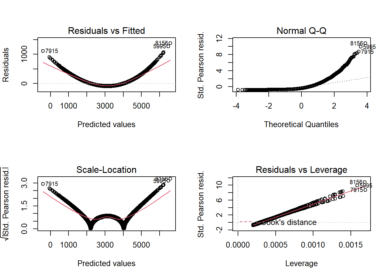
residuals <- residuals(fit)
par(mfrow=c(1,1))
plot(y=residuals,x=result.data$observed$Y) 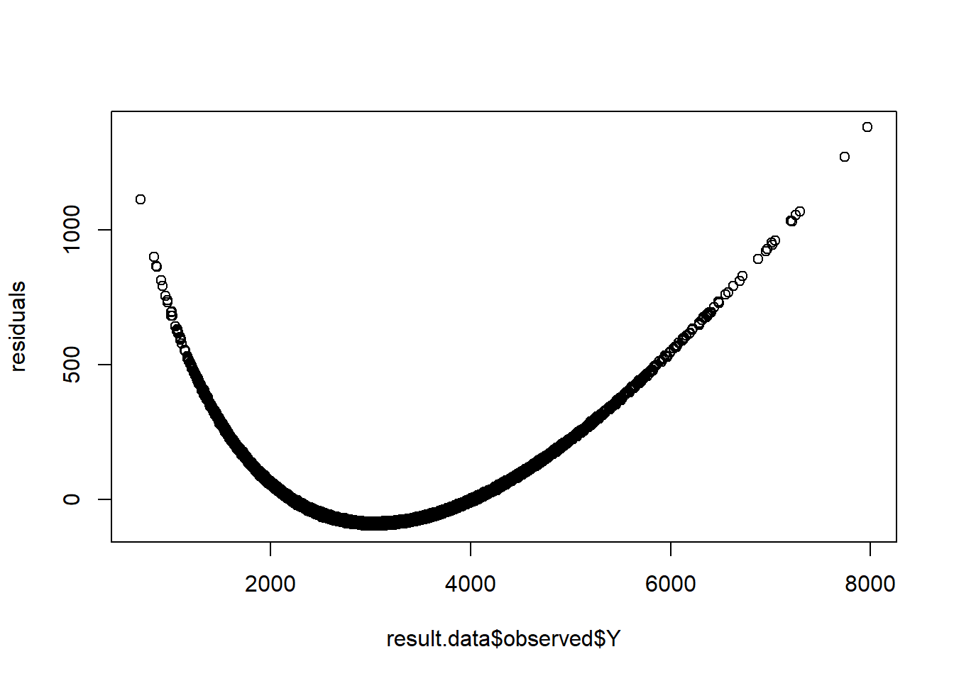
- Residual plot has a pattern!
- Indication that we may meed to reset the model-specification.
fit2 <- glm(Y ~ A + poly(L,2), family="gaussian", data=result.data$observed)
round(coef(fit2),2)
## (Intercept) A poly(L, 2)1 poly(L, 2)2
## 3087.50 0.92 90803.84 12753.21fit3 <- glm(Y ~ A + poly(L,3), family="gaussian", data=result.data$observed)
round(coef(fit3),2)## (Intercept) A poly(L, 3)1 poly(L, 3)2 poly(L, 3)3
## 3087.61 0.70 90803.92 12753.02 723.60