head(simdat)22 hdPS with a time-to-event outcome
22.1 Step 0: Analytic data
To demonstrate the use of the hdPS analysis with a time-to-event outcome, we will use a simulated dataset. The example is to explore the relationship between arthritis (binary exposure) and CVD (time-to-event outcome).
The simulated dataset contains information on 3,000 individuals with the following variables:
22.2 Step 1: Proxy sources
22.2.1 Data with investigator-specified covariates
Let us check the summary statistics of the investigator-specified covariates, stratified by the exposure variable (arthritis).
# Table 1
tab1 <- CreateTableOne(vars = c("age", "sex", "comorbidity"),
                       strata = "arthritis",
                       data = simdat,
                       test = FALSE)
print(tab1, showAllLevels = TRUE, noSpaces = TRUE, quote = FALSE, smd = TRUE)
#>                  Stratified by arthritis
#>                   level  No           Yes           SMD
#>   n                      2143         857
#>   age (mean (SD))        48.88 (9.53) 53.65 (10.03) 0.487
#>   sex (%)         Female 1189 (55.5)  592 (69.1)    0.283
#>                   Male   954 (44.5)   265 (30.9)
#>   comorbidity (%) No     1629 (76.0)  596 (69.5)    0.146
#>                   Yes    514 (24.0)   261 (30.5)

# Bivariate table
round(prop.table(table(arthritis = simdat$arthritis, CVD = simdat$cvd),
                 margin = 1)*100, 2)
#>          CVD
#> arthritis     0     1
#>       No  70.70 29.30
#>       Yes 43.52 56.48
22.2.2 Proxy data
In this example, we will use four data dimensions:
- 3-digit diagnostic codes from hospital database (diag)
- 3-digit procedure codes from hospital database (proc)
- 3-digit icd codes from physician claim database (msp)
- DINPIN from drug dispensation database (din)
table(dat.proxy$dim)
#>
#>  diag   din   msp  proc
#> 20000   269 44179   321
dat.proxy <- dat.proxy[order(dat.proxy$studyid),]
dat.proxy[5001:5010,]22.3 Step 2: Empirical covariates
The same as before, top 200 covariates with highest prevalence are chosen.
library(autoCovariateSelection)
id <- simdat$studyid

step1 <- get_candidate_covariates(df = dat.proxy, domainVarname = "dim",
                                  eventCodeVarname = "code",
                                  patientIdVarname = "studyid",
                                  patientIdVector = id,
                                  n = 200,
                                  min_num_patients = 20)
out1 <- step1$covars_data
head(out1)
22.4 Step 3: Recurrence
In this step, we generate a maximum of 3 binary recurrence covariates for each of the candidate proxy/code. We observed 401 recurrence covariates in this analysis.
22.4.1 Assessing recurrence of codes
all.equal(id, step1$patientIds)
#> [1] TRUE

step2 <- get_recurrence_covariates(df = out1,
                                   eventCodeVarname = "code",
                                   patientIdVarname = "studyid",
                                   patientIdVector = id)
out2 <- step2$recurrence_data
dim(out2)
#> [1] 3000  402
22.4.2 Recurrence covariates
vars.empirical <- names(out2)[-1]
head(vars.empirical)
#> [1] "rec_diag_C44_once" "rec_diag_C81_once" "rec_diag_C83_once"
#> [4] "rec_diag_E08_once" "rec_diag_E09_once" "rec_diag_E10_once"
22.4.3 Merging all recurrence covariates with the analytic dataset
hdps.data <- merge(simdat, out2, by = "studyid", all.x = T)
dim(hdps.data)
#> [1] 3000  408
22.5 Step 4: Prioritize
The Bross formula requires the exposure, outcome, and proxy covariates to be binary. With the time-to-event outcome, we will use Cox-PH with LASSO regularization to prioritize the empirical covariates. The hyperparameter (\(\lambda\)) will be selected using 5-fold cross-validation.
22.5.1 Hyperparameter tuning
# Formula with only empirical covariates
formula.out <- as.formula(paste("Surv(follow_up, cvd) ~ ",
                                paste(vars.empirical, collapse = " + ")))

# Model matrix for fitting Cox with LASSO regularization
X <- model.matrix(formula.out, data = hdps.data)[,-1]
Y <- as.matrix(data.frame(time = hdps.data$follow_up, status = hdps.data$cvd))

# Detect the number of cores
n_cores <- parallel::detectCores()

# Create a cluster of cores
cl <- makeCluster(n_cores - 1)

# Register the cluster for parallel processing
registerDoParallel(cl)

# Hyperparameter tuning with 5-fold cross-validation
set.seed(123)
fit.lasso <- cv.glmnet(x = X, y = Y, nfolds = 5, parallel = T, alpha = 1,
                       family = "cox")
stopCluster(cl)

plot(fit.lasso)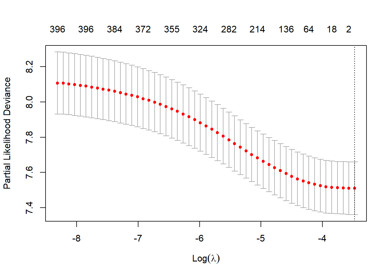
## Best lambda
fit.lasso$lambda.min
#> [1] 0.03093478
22.5.2 Variable ranking based on Cox-LASSO
empvars.lasso <- coef(fit.lasso, s = fit.lasso$lambda.min)
empvars.lasso <- data.frame(as.matrix(empvars.lasso))
empvars.lasso <- data.frame(vars = rownames(empvars.lasso),
                            coef = empvars.lasso)
colnames(empvars.lasso) <- c("vars", "coef")
rownames(empvars.lasso) <- NULL

# Number of non-zero coefficients
table(empvars.lasso$coef != 0)
#>
#> FALSE
#>   401
Since proxies were random and unrelated to the simulated data, LASSO produced all zero coefficients. Let choose an arbitrary value as to demonstrate the process of variable selection.
empvars.lasso <- coef(fit.lasso, s = exp(-6))
empvars.lasso <- data.frame(as.matrix(empvars.lasso))
empvars.lasso <- data.frame(vars = rownames(empvars.lasso),
                            coef = empvars.lasso)
colnames(empvars.lasso) <- c("vars", "coef")
rownames(empvars.lasso) <- NULL
head(empvars.lasso)
# Number of non-zero coefficients
table(empvars.lasso$coef != 0)
#>
#> FALSE  TRUE
#>    71   330
22.5.3 Rank empirical covariates
Now we will rank the empirical covariates based on absolute value of log hazard ratio.
empvars.lasso$coef.abs <- abs(empvars.lasso$coef)
empvars.lasso <- empvars.lasso[order(empvars.lasso$coef.abs, decreasing = T),]
head(empvars.lasso)
22.6 Step 5: Covariates
We used all investigator-specified covariates and the top 200 empirical covariates for the PS model. Again, this is a simplistic scenario where we only consider the main effects of the covariates.
# Investigator-specified covariates
investigator.vars <- c("age", "sex", "comorbidity")

# Top 200 empirical covariates section based on Cox-LASSO
empirical.vars.lasso <- empvars.lasso$vars[1:200]

# Investigator-specified and empirical covariates
vars.hsps <- c(investigator.vars, empirical.vars.lasso)
head(vars.hsps)
#> [1] "age"               "sex"               "comorbidity"
#> [4] "rec_diag_V03_once" "rec_diag_S24_once" "rec_diag_W61_once"
22.7 Step 6: Propensity score
22.7.1 Create propensity score formula
ps.formula <- as.formula(paste0("I(arthritis == 'Yes') ~ ",
                                paste(vars.hsps, collapse = "+")))
22.7.2 Fit PS model
require(WeightIt)
W.out <- weightit(ps.formula,
                    data = hdps.data,
                    estimand = "ATE",
                    method = "ps",
                  stabilize = T)
22.7.3 Obtain PS
hdps.data$ps <- W.out$ps22.7.4 Obtain weights
hdps.data$w <- W.out$weights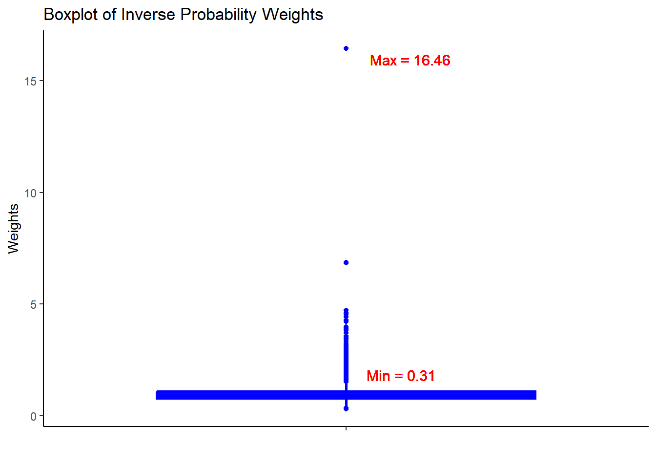
22.7.5 Assessing balance
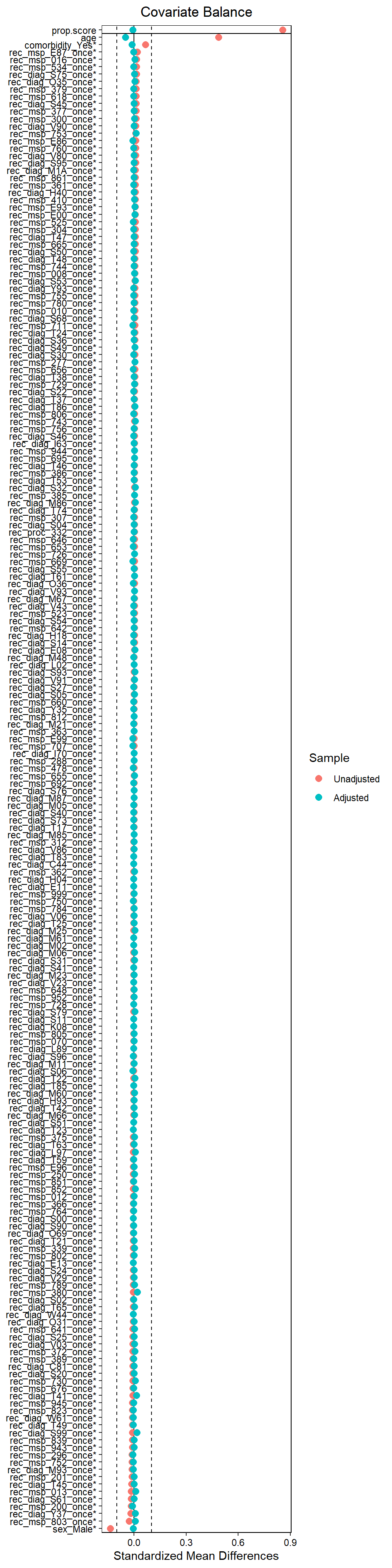
22.8 Step 7: Association
22.8.1 Obtain HR
library(survival)
library(Publish)
fit.hdps <- coxph(Surv(follow_up, cvd) ~ arthritis,
                  weights = w,
                  data = hdps.data)
publish(fit.hdps, pvalue.method = "robust", confint.method = "robust",
        print = F)$regressionTable[1:2,]
22.8.2 Obtain HR with survey package
library(survey)
# Create a design
svy.design <- svydesign(id = ~1, weights = ~w, data = hdps.data)

# Model
fit.hdps1 <- svycoxph(Surv(follow_up, cvd) ~ arthritis,
                      design = svy.design)
publish(fit.hdps1, print = F)$regressionTable[1:2,]
#> Independent Sampling design (with replacement)
#> svydesign(id = ~1, weights = ~w, data = hdps.data)