25  Time-dependent exposure

25.1 Time-dependent Cox regression

Let us start with an example of exploring the relationship between disease-modifying drugs (DMDs) for multiple sclerosis and long-term mortality. The DMD exposure is a time-dependent variable, and the mortality outcome is a time-to-event outcome. Employing Cox proportional hazards models with time-varying exposure to DMDs can address immortal time bias in this example.

Time-dependent exposure

• Time-dependent Cox regression with time-varying exposure can help mitigate immortal time bias.
• The hdPS approach is used to deal with residual confounding with a binary ‘time-fixed’ treatment
• With a ‘time-dependent’ exposure, implementing the hdPS in conjunction with the time-dependent Cox regression presents a methodological and practical challenge.

See the associated article for more details (Hossain et al. 2025).

25.2 Nested case-control (NCC)

The nested case-control (NCC) design is a well-established method for addressing immortal time bias with a time-dependent exposure. The NCC framework provides a robust alternative for addressing immortal time bias, while allowing for the integration of hdPS analysis to minimize the residual confounding bias.

(Austin et al. 2012; Ernster 1994; Hossain et al. 2024)

NCC

• Match subjects who experienced the event of interest (called cases) to a subset of event-free subjects (called controls) using incidence density sampling
• Some controls could later become cases themselves and also serve as controls for other cases
• Four controls per case has been shown to provide near-optimal statistical efficiency without the need for the full cohort analysis

25.3 hdPS in the NCC framework

The time-dependent exposure status becomes a time-independent exposure variable in the NCC analysis. Hence, we could implement the hdPS technique in the NCC framework to deal with residual confounding bias.

(Hossain et al. 2025)

25.3.1 Step 0: Analytic data

To demonstrate the use of hdPS analysis with a time-dependent exposure, we will use a simulated dataset. This example explores the relationship between exposure to disease-modifying drugs (DMDs) for multiple sclerosis and all-cause mortality.

25.3.1.1 Dataset with time-dependent exposure

head(simdat)

25.3.1.2 NCC with 4 control per case

Let us use the nested case-control (NCC) design with 4 controls per case. The ccwc function from the Epi package is used to create the nested case-control dataset. The ccwc function requires the following arguments:

• origin: The time origin for the study
• entry: The time of entry into the study
• exit: The follow-up time
• fail: The event of interest
• controls: The number of controls per case
• match: The variables to match on

library(Epi)
set.seed(100)

dat.ncc <- ccwc(
  origin = 0,
  entry = 0,
  exit = follow_up,
  fail = mortality_outcome,
  controls = 4, 
  match = list(ses, cci, year),
  include = list(id, follow_up, mortality_outcome, anyDMD, yrs_anyDMD, 
                 sex, age),
  data = simdat,
  silent = T
  )

# Drop those experienced the event before being exposed
dat.ncc$anyDMD[dat.ncc$yrs_anyDMD > dat.ncc$Time] <- NA
dat.ncc <- dat.ncc[complete.cases(dat.ncc$anyDMD),]

dat.ncc[1:10,]

# Rows
dim(simdat)
#> [1] 19000    10
dim(dat.ncc)
#> [1] 14370    14

# Mortality status
table(simdat$mortality_outcome)
#> 
#>     0     1 
#> 15947  3053
table(dat.ncc$Fail)
#> 
#>     0     1 
#> 11317  3053

25.3.2 Step 1: Proxy sources

In this example, we will use four data dimensions:

• 3-digit diagnostic codes from hospital database (diag)
• 3-digit procedure codes from hospital database (proc)
• 3-digit icd codes from physician claim database (msp)
• DINPIN from drug dispensation database (din)

table(dat.proxy$dim)
#> 
#>  diag   din   msp  proc 
#> 10000   125 22135   158

25.3.3 Step 2: Empirical covariates

library(autoCovariateSelection)
id <- simdat$id

step1 <- get_candidate_covariates(df = dat.proxy, domainVarname = "dim", 
                                  eventCodeVarname = "code", 
                                  patientIdVarname = "id", 
                                  patientIdVector = id, 
                                  n = 1000, 
                                  min_num_patients = 20)
out1 <- step1$covars_data
head(out1)

25.3.4 Step 3: Recurrence

Let us generate the binary recurrence covariates.

all.equal(id, step1$patientIds)
#> [1] TRUE

# Assessing recurrence of codes
step2 <- get_recurrence_covariates(df = out1, 
                                   eventCodeVarname = "code", 
                                   patientIdVarname = "id",
                                   patientIdVector = id)
out2 <- step2$recurrence_data
dim(out2)
#> [1] 19000   454

# Recurrence covariates
vars.empirical <- names(out2)[-1]
head(vars.empirical)
#> [1] "rec_diag_H02_once" "rec_diag_H18_once" "rec_diag_H35_once"
#> [4] "rec_diag_H40_once" "rec_diag_H44_once" "rec_diag_I69_once"

25.3.4.1 Merging all recurrence covariates with the analytic dataset

hdps.data <- merge(dat.ncc, out2, by = "id", all.x = T)
dim(hdps.data)
#> [1] 14370   467

25.3.5 Step 4: Prioritize

We will use Cox-PH with LASSO regularization to prioritize the empirical covariates. The hyperparameter (\(\lambda\)) will be selected using 5-fold cross-validation.

25.3.5.1 Hyperparameter tuning

# Formula with only empirical covariates
formula.out <- as.formula(paste("Surv(Time, Fail) ~ ", 
                                paste(vars.empirical, collapse = " + ")))

# Model matrix for fitting Cox with LASSO regularization
X <- model.matrix(formula.out, data = hdps.data)[,-1]
Y <- as.matrix(data.frame(time = hdps.data$Time, status = hdps.data$Fail))

# Detect the number of cores
n_cores <- parallel::detectCores()

# Create a cluster of cores
cl <- makeCluster(n_cores - 1)

# Register the cluster for parallel processing
registerDoParallel(cl)

# Hyperparameter tuning with 5-fold cross-validation 
set.seed(123)
fit.lasso <- cv.glmnet(x = X, y = Y, nfolds = 5, parallel = T, alpha = 1, 
                       family = "cox")
stopCluster(cl)

plot(fit.lasso)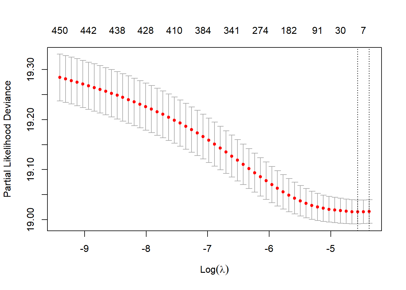

## Best lambda
fit.lasso$lambda.min
#> [1] 0.01042345

25.3.5.2 Variable ranking based on Cox-LASSO

empvars.lasso <- coef(fit.lasso, s = fit.lasso$lambda.min) 
empvars.lasso <- data.frame(as.matrix(empvars.lasso))
empvars.lasso <- data.frame(vars = rownames(empvars.lasso), 
                            coef = empvars.lasso)
colnames(empvars.lasso) <- c("vars", "coef")
rownames(empvars.lasso) <- NULL

# Number of non-zero coefficients
table(empvars.lasso$coef != 0)
#> 
#> FALSE  TRUE 
#>   442    11

Since proxies were random and unrelated to the simulated data, LASSO produced only 11 non-zero coefficients. Let choose an arbitrary value as to demonstrate the process of variable selection.

empvars.lasso <- coef(fit.lasso, s = exp(-6)) 
empvars.lasso <- data.frame(as.matrix(empvars.lasso))
empvars.lasso <- data.frame(vars = rownames(empvars.lasso), 
                            coef = empvars.lasso)
colnames(empvars.lasso) <- c("vars", "coef")
rownames(empvars.lasso) <- NULL
head(empvars.lasso)

# Number of non-zero coefficients
table(empvars.lasso$coef != 0)
#> 
#> FALSE  TRUE 
#>   196   257

25.3.5.3 Rank empirical covariates

Now we will rank the empirical covariates based on absolute value of log hazard ratio.

empvars.lasso$coef.abs <- abs(empvars.lasso$coef)
empvars.lasso <- empvars.lasso[order(empvars.lasso$coef.abs, decreasing = T),]
head(empvars.lasso)

25.3.6 Step 5: Covariates

We used all investigator-specified covariates and the top 200 empirical covariates for the PS model. Again, this is a simplistic scenario where we only consider the main effects of the covariates.

# Investigator-specified covariates
investigator.vars <- c("sex", "age")

# Top 200 empirical covariates section based on Cox-LASSO
empirical.vars.lasso <- empvars.lasso$vars[1:200]

# Investigator-specified and empirical covariates
vars.hsps <- c(investigator.vars, empirical.vars.lasso)
head(vars.hsps)
#> [1] "sex"               "age"               "rec_diag_T44_once"
#> [4] "rec_diag_O41_once" "rec_msp_793_once"  "rec_msp_459_once"

25.3.7 Step 6: Propensity score

25.3.7.1 Create propensity score formula

ps.formula <- as.formula(paste0("I(anyDMD == 'Yes') ~ ", 
                                paste(vars.hsps, collapse = "+")))

25.3.7.2 Fit PS model

require(WeightIt)
W.out <- weightit(ps.formula, 
                    data = hdps.data, 
                    estimand = "ATE",
                    method = "ps",
                  stabilize = T)

25.3.7.3 Obtain PS

hdps.data$ps <- W.out$ps

25.3.7.4 Obtain weights

hdps.data$w <- W.out$weights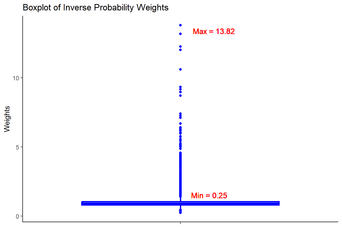

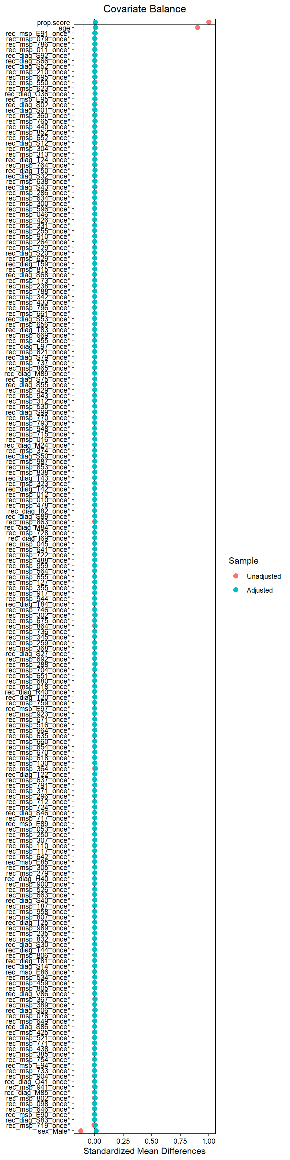
25.3.7.5 Assessing balance

library(survey)

# Balance checking for investigator-specified covariates
design.ipw <- svydesign(ids = ~id, weights = ~w, data = hdps.data)
tab.ipw <- svyCreateTableOne(vars = investigator.vars, 
                             strata = "anyDMD", 
                             data = design.ipw, 
                             test = F)
print(tab.ipw, smd = T) # Age and sex are balanced
#>                  Stratified by anyDMD
#>                   No               Yes             SMD   
#>   n                11035.4          3324.4               
#>   sex = Male (%)    3199.3 (29.0)   1007.3 (30.3)   0.029
#>   age (mean (SD))    45.58 (13.75)   45.67 (13.48)  0.007

25.3.8 Step 7: Association

25.3.8.1 Obtain HR

We can fit the Cox-PH model, adjusting for the matched strata.

library(survival)
library(Publish)
fit.hdps <- coxph(Surv(Time, Fail) ~ anyDMD + strata(Set), 
                  weights = w,
                  data = hdps.data)
publish(fit.hdps, pvalue.method = "robust", confint.method = "robust", 
        print = F)$regressionTable[1:2,]

25.3.8.2 Obtain HR with conditional logistic

For the NCC analysis, an alternative to the stratified Cox-PH model is to use the conditional logistic regression. The HR and SE from both models should be similar under the proportional hazards assumption.

(Liu et al. 2010)

fit.hdps1 <- clogit(Fail ~ anyDMD + strata(Set), 
                    weights = w, 
                    data = hdps.data, 
                    method = "efron")
publish(fit.hdps1, pvalue.method = "robust", confint.method = "robust", 
        print = F)$regressionTable[1:2,]

Austin, Peter C, Geoffrey M Anderson, Candemir Cigsar, and Andrea Gruneir. 2012. “Comparing the Cohort Design and the Nested Case–Control Design in the Presence of Both Time-Invariant and Time-Dependent Treatment and Competing Risks: Bias and Precision.” Pharmacoepidemiology and Drug Safety 21 (7): 714–24.

Ernster, Virginia L. 1994. “Nested Case-Control Studies.” Preventive Medicine 23 (5): 587–90.

Hossain, Md Belal, Huah Shin Ng, Feng Zhu, Helen Tremlett, and Mohammad Ehsanul Karim. 2025. “Simultaneously Dealing with Immortal Time Bias and Residual Confounding: A Case Study of a High-Dimensional Propensity Score Approach with a Nested Case–Control Framework in Multiple Sclerosis Research.” Pharmacoepidemiology and Drug Safety 34 (7): e70174.

Hossain, Md Belal, Hubert Wong, Mohsen Sadatsafavi, James C Johnston, Victoria J Cook, and Mohammad Ehsanul Karim. 2024. “Benefits of Repeated Matched-Cohort and Nested Case–Control Analyses with Time-Dependent Exposure in Observational Studies.” Statistics in Biosciences, 1–29.

Liu, Mengling, Wenbin Lu, Roy E Shore, and Anne Zeleniuch-Jacquotte. 2010. “Cox Regression Model with Time-Varying Coefficients in Nested Case–Control Studies.” Biostatistics 11 (4): 693–706.