3  Step 0: Analytic data

3.1 Creating Analytic data

3 cycles of NHANES datasets were - downloaded from the US CDC website - recoded for consistency, and - merged together to make an analytic data.

Details of data download process, and recoding and merging are discussed in Appendix.

flowchart LR
  A[NHANES] --> C1(2013-2014 cycle) --> ss1(10,175 \nparticipants)
  A --> C2(2015-2016 cycle) --> ss2(9,971 \nparticipants)
  A --> C3(2017-2018 cycle) --> ss3(9,254 \nparticipants)
  ss1 --> ss(7,585 \nafter \nimposing \neligibility \ncriteria)
  ss2 --> ss
  ss3 --> ss
  style A fill:#FFA500;
  style C1 fill:#FFA500;
  style C2 fill:#FFA500;
  style C3 fill:#FFA500;
  style ss1 fill:#FFA500;
  style ss2 fill:#FFA500;
  style ss3 fill:#FFA500;
  style ss fill:#FFA500;

Our study population was restricted to the U.S. population who were

• 20 years or older and
• not pregnant at the time of survey data collection, and
• who had available International Classification of Diseases (ICD) codes to ensure we can extract sufficient proxy information for the analysis (discussed in step 1).

To simplify the analysis, we only considered complete case data.

3.2 PS model (no proxies)

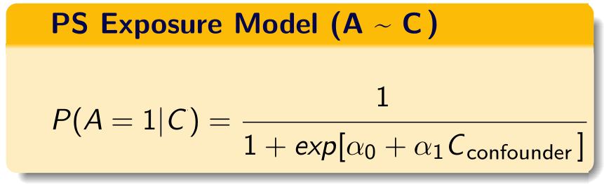
We build the propensity score model in this data using the investigator-specified covariates.

C = investigator-specified covariates.

Then the PS can be used as matching, weighting, stratifying variables, or as covariates (usually in deciles) in outcome model.

If you are somewhat unfamiliar with propensity score paradigm, look at tutorials dedicated towards that topic. There are additional tutorials also talking about propensity score weighting.

In our current context, we only talk about inverse probability weighting.

Tip

Results from propensity score analysis (through inverse probability weighting) with only investigator-specified covariates are shown in Propensity Score section.