11 Propensity score
Compare the measures of association with those obtained from a regular propensity score method, so that we can compare the estimates.
11.1 Fitting PS model to obtain OR
11.1.1 Create propensity score formula
covform <- paste0(investigator.specified.covariates, collapse = "+")
ps.formula <- as.formula(paste0("exposure", "~", covform))
ps.formula
#> exposure ~ age.cat + sex + education + race + marital + income +
#>     born + year + diabetes.family.history + medical.access +
#>     smoking + diet.healthy + physical.activity + sleep + uric.acid +
#>     protein.total + bilirubin.total + phosphorus + sodium + potassium +
#> globulin + calcium.total + systolicBP + diastolicBP + high.cholesterol- Only use investigator specified covariates to build the formula.
- During the construction of the propensity score model, researchers should consider incorporating additional model specifications, such as interactions and polynomials, if they are deemed necessary.
Propensity score models typically involve a greater number of covariates and incorporate other functional specifications (interactions) (Ho et al. 2007). In this context, overfitting is generally considered to be less worrisome as long as satisfactory overlap and balance diagnostics are achieved. This is because, some researchers suggest that propensity score model is meant to be descriptive of the data in hand, and should not be generalizabled (Judkins et al. 2007). However, there is a limit to it. Recent literature did suggest that propensity score model overfitting can lead to inflated variance of estimated treatment effect estimate (Schuster, Lowe, and Platt 2016). While the standard errors of the beta coefficients from the propensity score model are not typically a primary concern, it is generally advisable to examine them as part of the diagnostics process for assessing the propensity score model (Platt et al. 2019). Specifically, techniques like double cross-fitting have demonstrated promise in minimizing the aforementioned impact (Karim 2023).
11.1.2 Fit PS model
require(WeightIt)
W.out <- weightit(ps.formula,
                    data = hdps.data,
                    estimand = "ATE",
method = "ps")- Use that formula to estimate propensity scores.
- In this demonstration, we did not use
stabilize = TRUE. However, stabilized propensity score weights often reduce the variance of treatment effect estimates.
11.1.3 Obtain PS
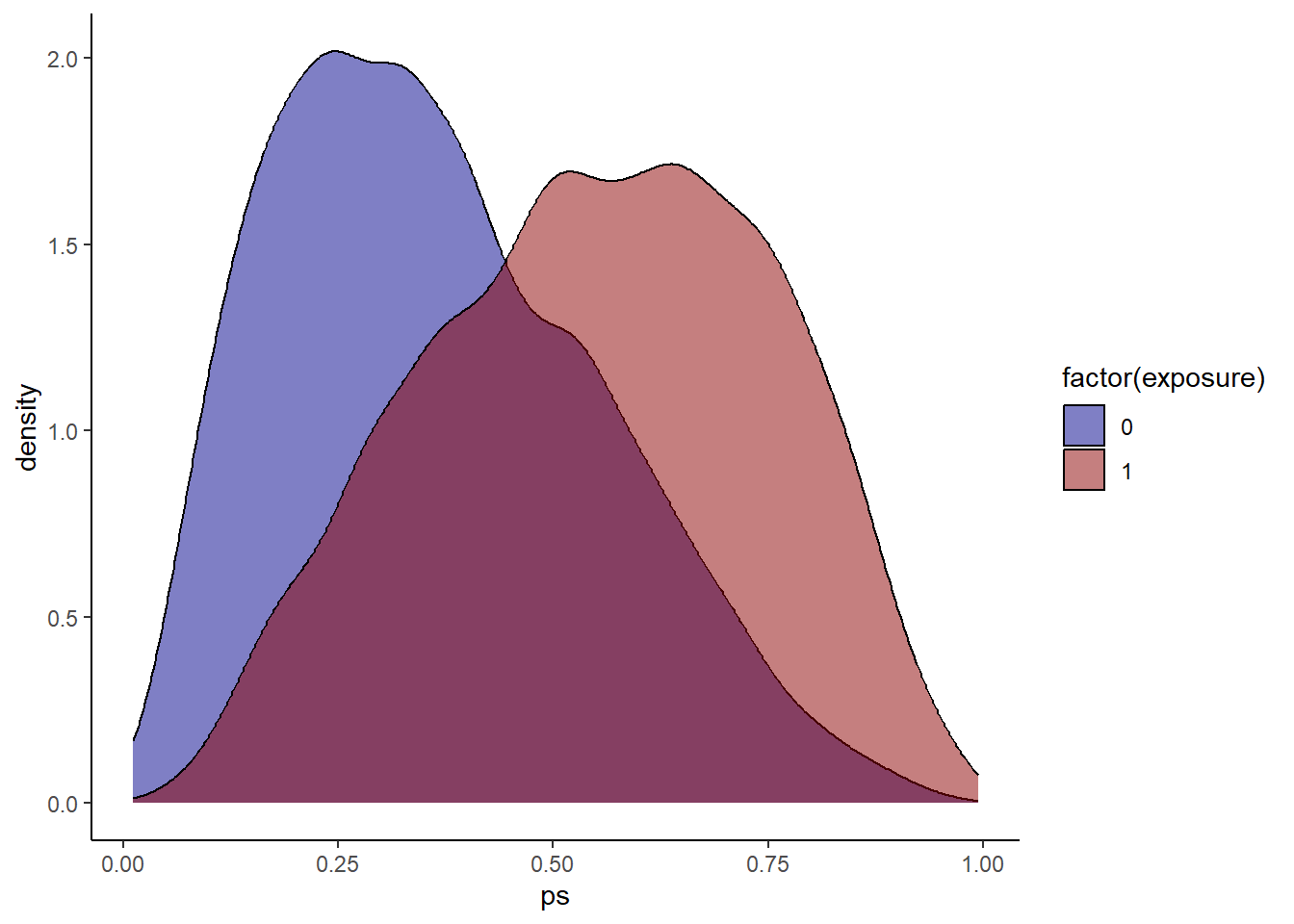
Check propensity score overlap in both exposure groups. Similar as before?
11.1.4 Obtain Weights
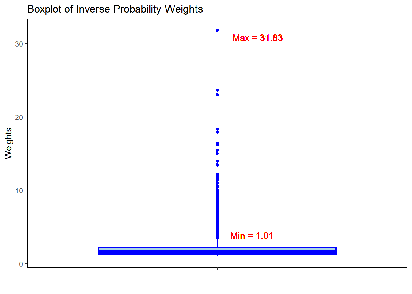
- Check the summary statistics of the weights to assess whether there are extreme weights. Less extreme weights now?
11.1.5 Assessing balance
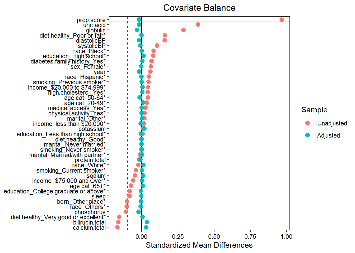
- Assess balance against SMD 0.1. Still balanced?
- Predictive measures such as c-statistics are not helpful in this context (Westreich et al. 2011): “use of the c-statistic as a guide in constructing propensity scores may result in less overlap in propensity scores between treated and untreated subjects”!
11.1.6 Set outcome formula
out.formula <- as.formula(paste0("outcome", "~", "exposure"))
out.formula
#> outcome ~ exposure
We are again using a crude weighted outcome model here.
11.1.7 Obtain OR from unadjusted model
fit <- glm(out.formula,
            data = hdps.data,
            weights = W.out$weights,
            family= binomial(link = "logit"))
fit.summary <- summary(fit)$coef["exposure",
                                 c("Estimate",
                                   "Std. Error",
                                   "Pr(>|z|)")]
fit.ci <- confint(fit, level = 0.95)["exposure", ]
fit.summary_with_ci.ps <- c(fit.summary, fit.ci)
round(fit.summary_with_ci.ps,2)
#>   Estimate Std. Error   Pr(>|z|)      2.5 %     97.5 %
#>       0.68       0.04       0.00       0.61       0.76
11.2 Fitting crude model to obtain OR
Here we estimate the crude association between the exposure and the outcome.
fit <- glm(out.formula,
            data = hdps.data,
            family= binomial(link = "logit"))
fit.summary <- summary(fit)$coef["exposure",
                                 c("Estimate",
                                   "Std. Error",
                                   "Pr(>|z|)")]
fit.ci <- confint(fit, level = 0.95)["exposure", ]
fit.summary_with_ci.crude <- c(fit.summary, fit.ci)
round(fit.summary_with_ci.crude,2)
#>   Estimate Std. Error   Pr(>|z|)      2.5 %     97.5 %
#>       0.73       0.05       0.00       0.63       0.84
No adjustment at all!